Stanford-CS224n

CS224n

学习Stanford的CS224n Natural Language Processing with Deep Learning。(课程链接)

[TOC]

Lecture 1. Introduction and word vector

---

introduction

• basic和key mothods：RNN attention transformers
• 理解对人类自然语言理解中问题
• 用PyTorch构建模型，解决word meaning，dependency parsing，machine translation，QA等问题

NLP levels

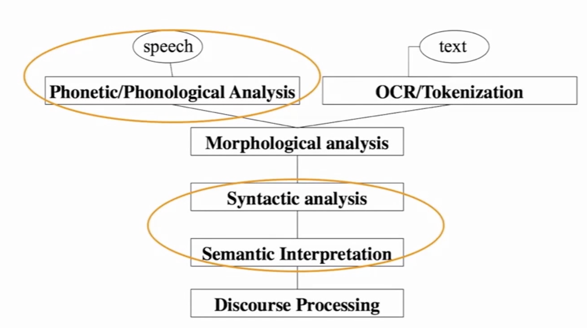
输入speech text->单词分析->句法分析->语义理解->上下文处理

human language

language is discrete/symbolic/categorical signaling system

• rocket=🚀 violin=🎻
• love loooove

人类语言是一套符号系统，深度学习领域将大脑视为有连续的激活模式。

deep learning

• machine learning：由人类审视一个特定的问题，找出问题中的关键要素，设计useful features/signals，使用这些features解决问题，机器做数值优化。大部分工作是人类的数据分析。
  • 手动设计的特征过于具体，长时间设计和调整
• deep learning：表征学习的一个分支，输入原始的真实世界信号，机器自己学习特征，可以得到多层的learned representations。
  • deep learning的特征适应性强，训练快，可以灵活通用地学习
  • 海量数据+算力提升

Word Vector (represent the meaning of a word)

meaning

• 用一个词、词组表示的概念
• 一个人想用语言、符号表示的想法
• 表达在文学、艺术作品等方面的思想

理解meaning的linguistic way：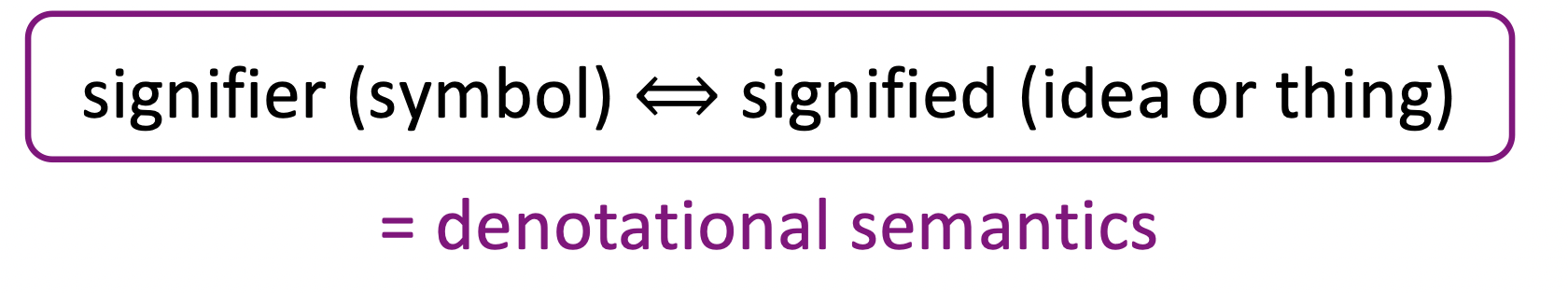

（指称语义）

how do we have usable meaning in a computer

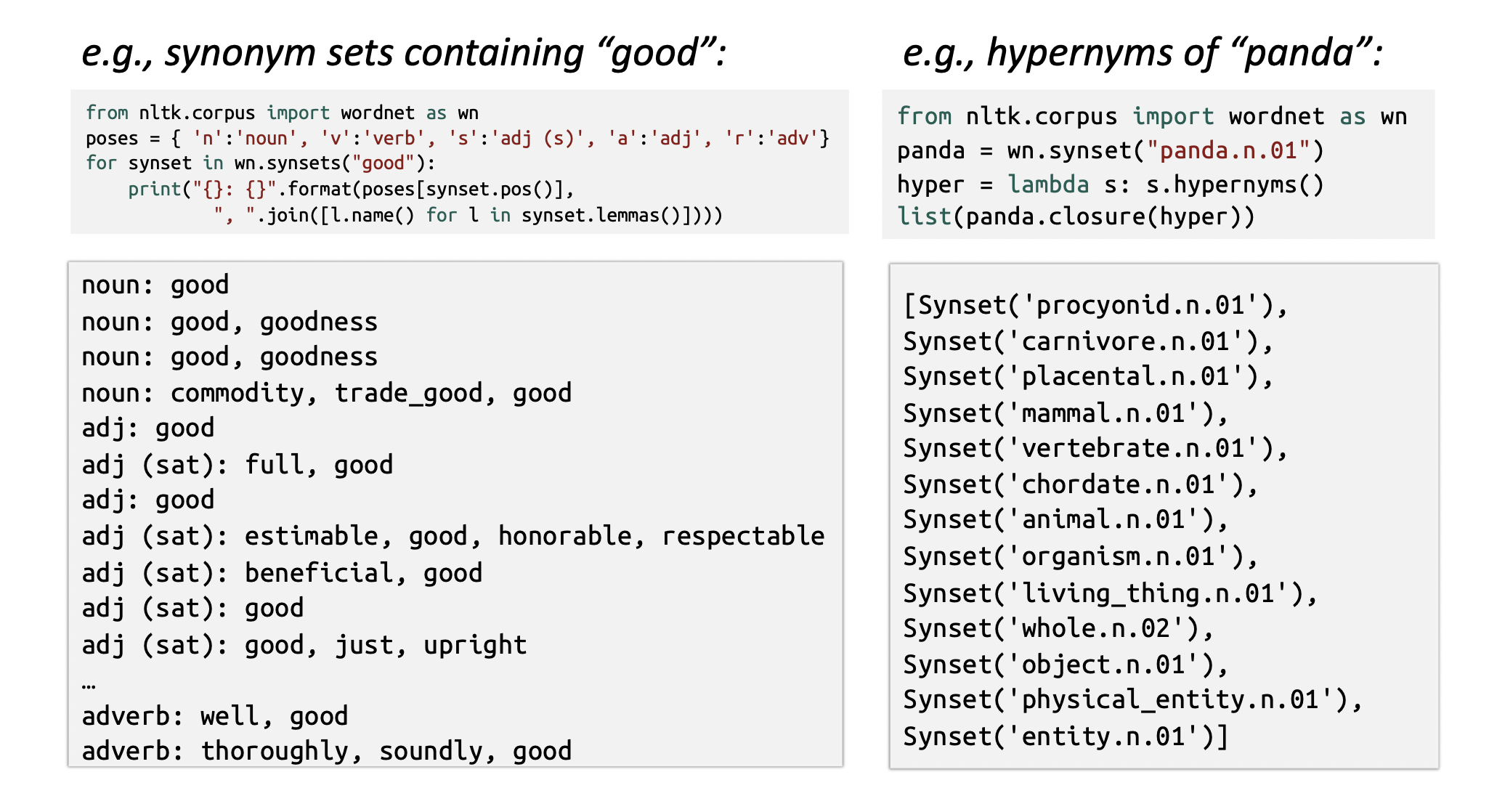
common NLP solution：WordNet，包含同义词集合和上位词(例如”is a”关系)的列表的词典。

• 同义词和上位词
  

problems with resources like WordNet

• 作为资源使用很好，但忽略了细微差别（missing nuance）
  • e.g. proficient 和 good是同义词，但需要结合上下文
• 难以持续更新，缺乏单词的新含义
• 比较主观subjective
• 需要人力物力创建和调整词库
• 没有单词相似度的概念

representing words as discrete symbols

在传统NLP中，word被视为离散符号，被表示为one-hot vec。

• problems：
  • 所有的vec都正交
  • one-hot vec没有相似度的概念
  • 向量维度太大
• solution：
  • 使用类似wordnet的list来表示相似度，但有不完整性
  • 学习使用real-value vec本身来编码计算相似度

Representing words by their context

• 分布式语义（distributional semantics）：word的语义由经常出现在其附近的单词给出。
• 当一个单词w出现在一段文本中时，在一个固定大小的窗口内co-occur的单词就是w的上下文词，使用w的contexts来构建w的表示

word vector/word embedding/word representation

为每个单词构建dense vec，使其与context中出现的单词的dense vec相似。

• word2vec
• glove
• sanjiv aurora’s paper

word2vec（Mikolov et al. 2013）

一个学习word vec的框架：

• 有一个大的语料库corpus
• 词汇表中的每个单词用一个vec表示
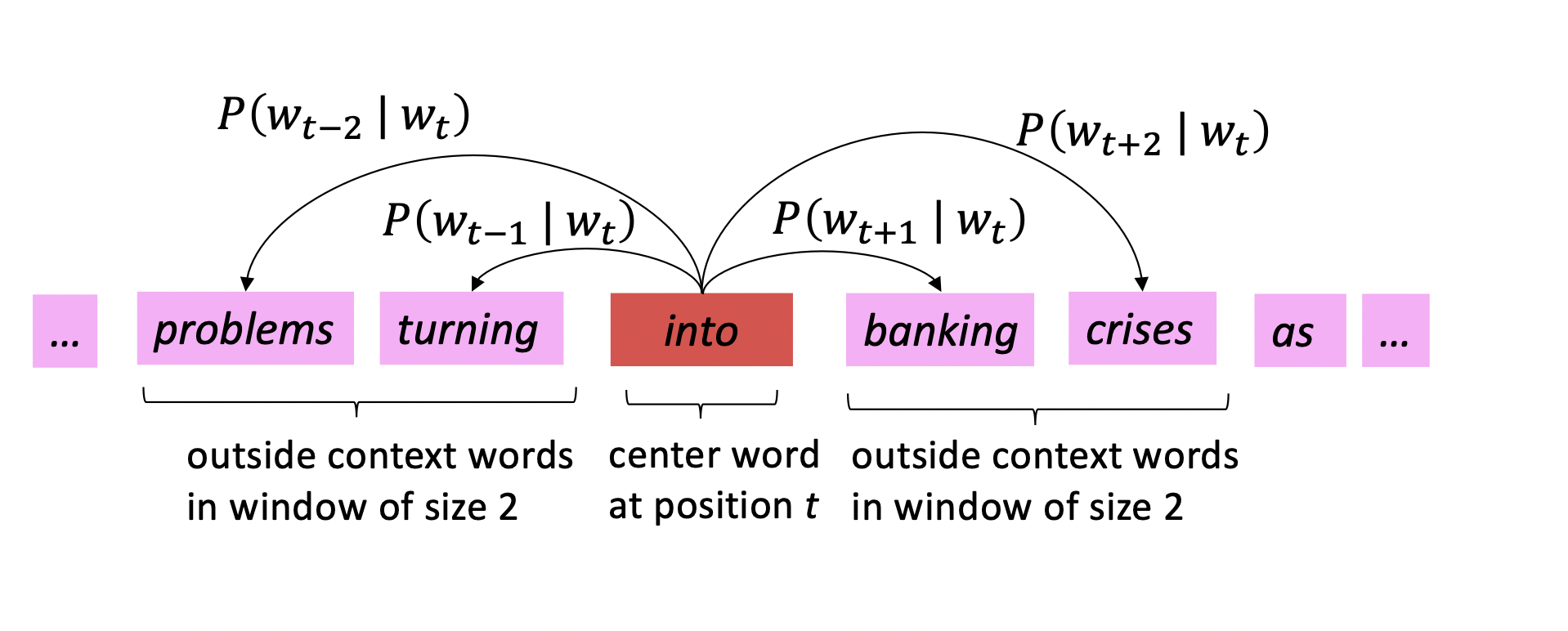
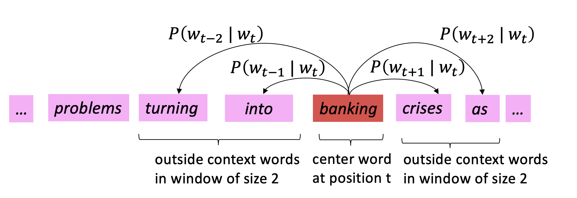
• 对text中的每个位置t，有一个中心词$c$和一些上下文（context/outside）词$o$
• 用c和o词向量的相似性来计算给定$c$时$o$的概率$P(o|c)$
• 不断调整词向量，最大化这个概率$P(o|c)$

word2vec objective func

对每个位置$t=1,\cdots,T$，在一个大小为$m$的固定窗口内预测context words，给定中心词$w_j$，有
$Likelihood=L(\theta)=\Pi^T_{t=1}\Pi_{-m\le j\le m,j\neq 0}P(w_{t+j}|w_t;\theta)$

目标函数为：
$J(\theta)=-\frac{1}{T}\Sigma_{t=1}^T\Sigma_{-m\le j\le m,j\neq 0}\ log\ P(w_{t+j}|w_t;\theta)$

经典的$\Pi$通过log变成$\Sigma$，最小化目标函数->最大化似然函数

• 如何计算 $P(w_{t+j}|w_t;\theta)$
  • $v_w$：w为中心词的vec
  • $u_W$：w是上下文词的vec
  • 则$P(o|c)=\frac{exp(u_o^Tv_c)}{\Sigma_{w\in V}exp(u_w^Tv_c)}$，向量点积越大即相似度越高

此处使用Softmax:$\mathbb{R}^n->(0,1)^n$将点积得到的任意值$x_i$映射到概率分布$p_i$

梯度下降

在负梯度上take small step

• Gradient

  $$\begin{aligned} \frac{\partial }{\partial v_c}log\ P(o|c) &= \frac{\partial }{\partial v_c}(log\ exp(u^T_ov_c)-\Sigma_{w\in V}exp(u_w^Tv_c)) \\ &= \frac{\partial }{\partial v_c}(u_o^Tv_c-log\ \Sigma_{w\in V}exp(u_w^Tv_c)) \\ &= u_o - \frac{\Sigma_{w\in V}exp(u_w^Tv_c)u_w}{\Sigma_{w\in V}exp(u_w^Tv_c)} \\ &= u_o - \Sigma_{w\in V}\frac{exp(u_w^Tv_c)}{\Sigma_{w\in V}exp(u_w^Tv_c)}u_w \\ &= u_o - \Sigma_{w\in V}P(w|c)u_w \\ &= observed - expected \end{aligned}$$

• Update equation
  $\theta^{new} = \theta^{old} - \alpha \bigtriangledown_\theta J(\theta)$

  while True:
      theta_grad = evaluate_gradient(J, corpus, theta)
      theta = theta - alpha * theta_grade

---

Lecture 2. Word Vectors 2 and Word Window Classification

stochastic gradient descent（SGD）

• 问题：$J(\theta)$是语料库中所有window的函数，梯度计算开销很大
• 方案：SGD，随机采样windows，在每个window或batch后update

while True:
    window = sample_window(corpus)
    theta_grad = evaluate_gradient(J, window, theta)
    theta = theta - alpha * theta_grade

more details

两个向量：更好优化，center vec和context vec最终会是相似的

两类模型：

• Skip-Grams: 给定中心词预测上下文
• Continuous Bag of Words: 给定（bag of）上下文词，预测中心词

其他训练策略：

• negative sampling
• negative sampling for naive softmax

word2vec 比较crude，很大程度上忽略了词的具体位置

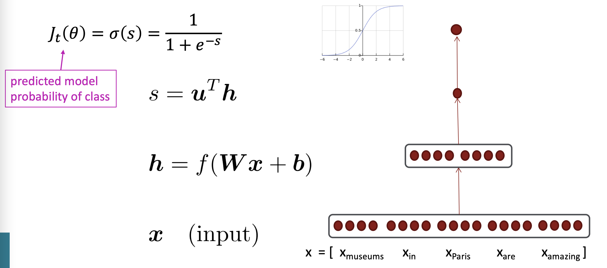
skip-gram model with negative sampling（HW2）

$P(o|c)=\frac{exp(u_o^Tv_c)}{\Sigma_{w\in V}exp(u_w^Tv_c)}$中分母的计算开销过大

• Main idea：用true pair（中心词与其上下文窗口中的词）与几个noise pair（中心词与随机词）训练二元逻辑回归

• maximize目标函数：$J(\theta)=\frac{1}{T}\Sigma^T_{t=1}J_t(\theta)$
  $J_t(\theta)=log\ \sigma(u_o^Tv_c)+\Sigma^k_{i=1}\mathbb{E}_{j\sim P(w)}[log\ \sigma(-u^T_jv_c)]$
  $\sigma(x)=\frac{1}{1+e^{-x}}$

maximize前半部分真实上下文词的概率，minimize后半部分负采样随机词的概率

负采样方案：$P(w)=U(w)^{3/4}/Z$，$U(w)$是unigram分布，用幂提升罕见词的采样概率，$Z$为归一化。

why not capture co-ocurrence counts directly?

构建co-occurence matrix $X$的两种方法：

• 窗口windows：与w2v类似，使用中心词附近的window，捕获句法和语义信息
• 全文full document：窗口大小设为文章长度，常用于信息检索方法中，如Latent Semantic Analysis

问题：

• 词表变大则向量维度也要增大，但向量很稀疏
• 分类模型也会遭遇稀疏的问题，鲁棒性差

需要使用low-dim的dense matrix。

Classic Method Dimensionality Reduction on X（HW1）

用SVD分解$X$为$U\Sigma V^T$，$U$和$V$对应行和列的正交基。

为了减少尺度，可以保留$\Sigma$对角阵中的topK最大值，并保留$U,V$对应的行列。

• 直接对原始的count做SVD效果很差，需要对数字进行调整：
  • 取log
  • 取$min(X,\delta)$
  • 忽略虚词的count
• 使用斜坡ramped window，对更近的词计更大的count
• 用Pearson相关系数（Pearson Correlation Coefficient）代替count，然后将负值置零

Towards GloVe：Count based vs direct prediction

• count based：基于co-occurence
  • LSA、HAL、COALS、Hellingger-PCA
  • 训练快；有效使用统计数据
  • 主要用于捕获词相似性；过分重视count大的数据
• direct prediction：定义概率分布，根据概率预测词
  • Skip-gram/CBOW、NNLM、HLBL、RNN
  • 规模跟corpus大小有关；没有有效利用统计数据（采样和窗口）
  • 提高了在其他任务上的表现；可以捕获相似度之外更复杂的信息

Encoding meaning in vector differences

结合两种方法，在神经网络中引入count矩阵

核心思想：co-orrurrence概率之比可以编码meaning components

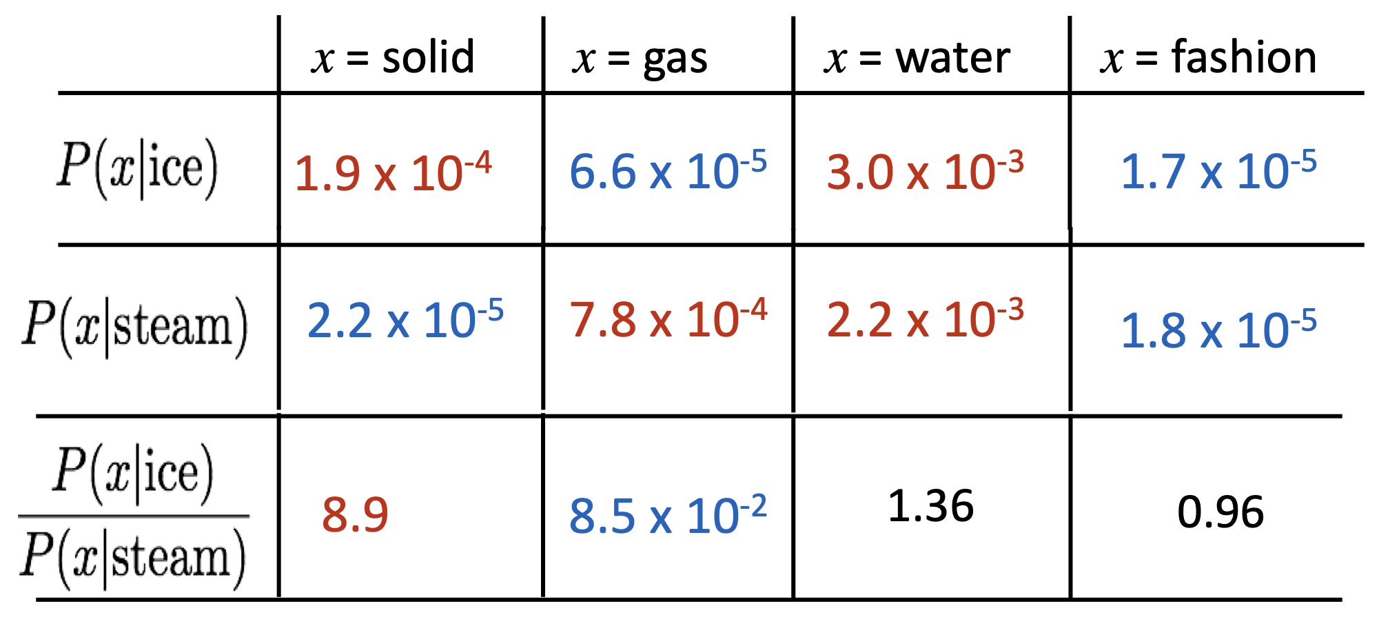
单一的概率并非重点，概率的比值更能反映(linear) meanning component。

关键：$\frac{P(x|a)}{P(x|b)}$如何在词向量空间中捕获？

• 用向量的点积表示co-occurence 概率的对数
• $w_i\cdot w_j = log P(i|j)$
• $w_x\cdot (w_a - w_b)\frac{P(x|a)}{P(x|b)}$
• $J=\Sigma^V_{i,j=1}f(X_{ij})(w_i^T\tilde w_j+b_i+\tilde b_j-log X_{ij})^2$
  $f$限制了常见词的count

how to evaluate word vectors

• Intrinsic
  • 在特定和中间子任务上评估
  • 评估运算很快
  • 有助于理解整个系统
  • 在用于实际任务前不清楚是否有用
• Extrinsic
  • 在实际任务上评估
  • 通常需要更长时间（任务更大）
  • 不清楚系统整个系统的问题所在

word sense and word sense ambiguity

• 多义的word 和 一一对应的word vec相悖

imporving word representations via global context and multiple word prototypes（Huang et al. 2012）

对常用词的所有context聚类，从而得到一些表示不同含义的簇。

划分并不明确且存在重叠。

Linear Algebraic Structure of Word Senses, with Applications to Polysemy

• 单词的不同含义以加权的线性形式叠加：
  $v_w=\Sigma\alpha_iv_{w_i}$
  $\alpha_i=\frac{f_i}{\Sigma f_j}$
• 实际上，用稀疏编码Sparse coding的思想，不同维度表示了不同的含义，所以weighted-avg对不同含义的维度损失很小。

Lecture 3. Backprop and Neural Networks

matrix calculus

gradient

• 单输出多输入的函数$f(\mathbf{x})=f(x_1,\dots,x_n)$
• 梯度gradient是关于每个输入的偏导数partial derivatives的向量$\frac{\partial f}{\partial x}=[\frac{\partial f}{\partial x_1},\dots,\frac{\partial f}{\partial x_n}]$

Jacobian Matirx: Generalization of the Gradient

• 多输出多输入的函数$\mathbf{f(x)}=[f_1(x_1,\dots,x_n),\dots,f_m(x_1,\dots,x_n)]$
• Jacobian mat是$m\times n$的矩阵：
  $\mathbf{\frac{\partial f}{\partial x}}=
  \begin{bmatrix}
  \frac{\partial f_1}{\partial x_1} & \dots & \frac{\partial f_1}{\partial x_n} \\
  \vdots & \ddots & \vdots \\
  \frac{\partial f_m}{\partial x_1} & \dots & \frac{\partial f_m}{\partial x_n} \\
  \end{bmatrix}$

chain rule

多变量的链式法则：乘Jacobian mat

example：NER

• 找出文本中的实体并分类
  
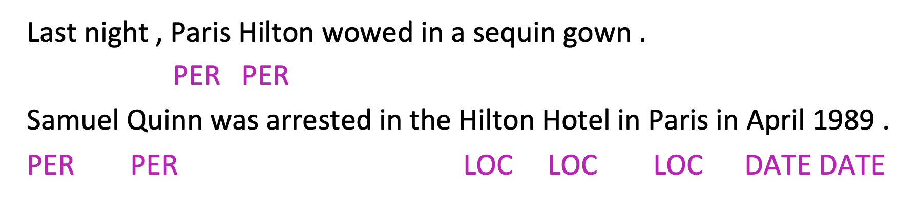
• Idea：通过上下文窗口来对每个词分类，对每个类训练logistic分类器
  

计算梯度

• 计算$\frac{\partial s}{\partial \mathbf{b}}$
  
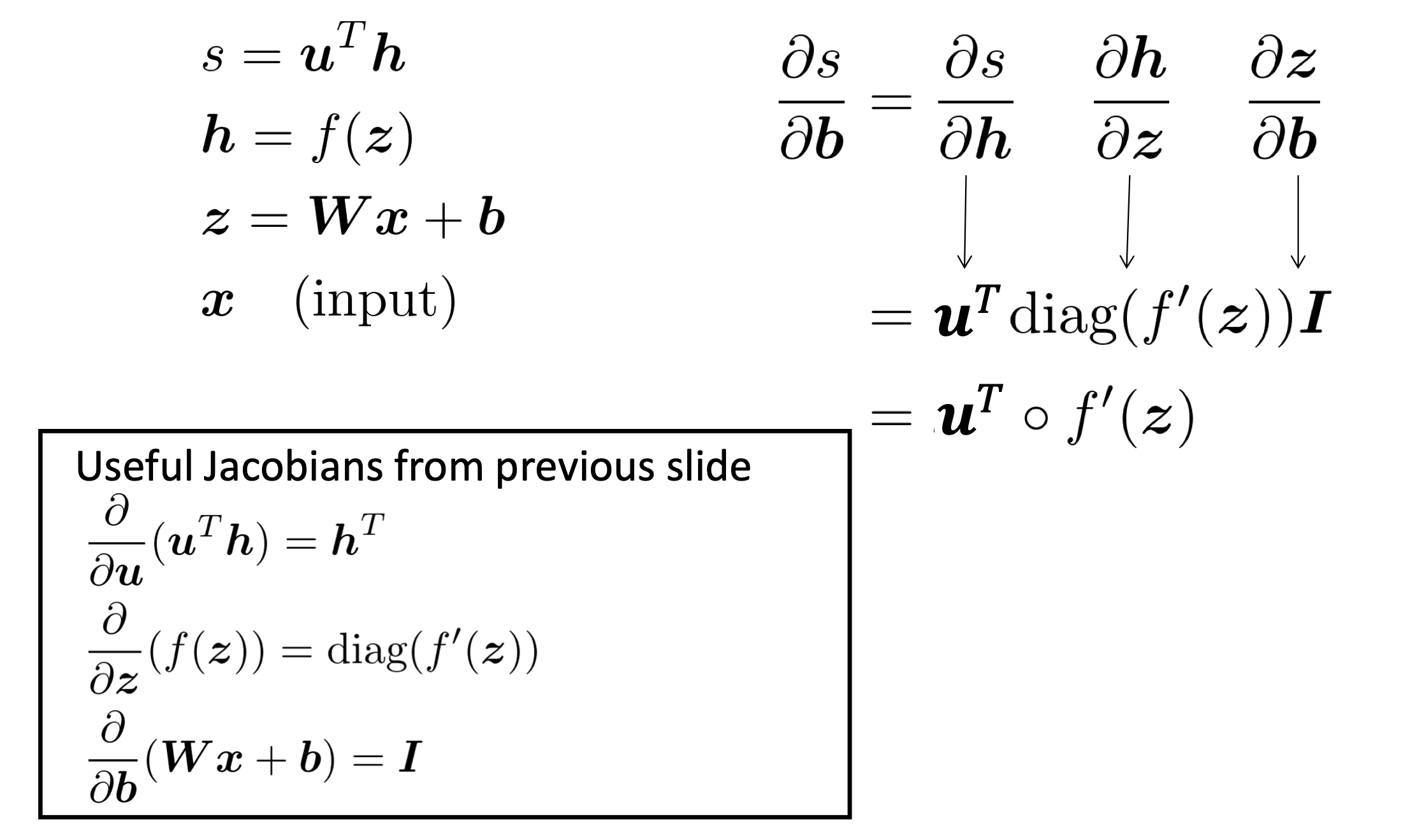
• 计算$\frac{\partial s}{\partial \mathbf{W}}$
  与上述过程相似，其中前两项是一致的，无需重复计算
  $\frac{\partial s}{\partial \mathbf{W}}=\delta\frac{\partial z}{\partial \mathbf{W}}$
  $\delta=\frac{\partial s}{\partial \mathbf{h}}\frac{\partial \mathbf{h}}{\partial z}=\mathbf{u}^T\circ f’(z)$是local error signal

derivative with respect to Matrix: output shape

• 输出大小为1，输入大小为$n\times m$.
• 从数学角度，输出应该为$1\times nm$
• 但为了方便更新参数，其shape应为$n\times m$

$\frac{\partial s}{\partial \mathbf{W}}=\delta^Tx^T$，transpose可以解决shape的问题

Lecture 4. Dependency Parsing

---

Dependency Parsing

constituency Parsing

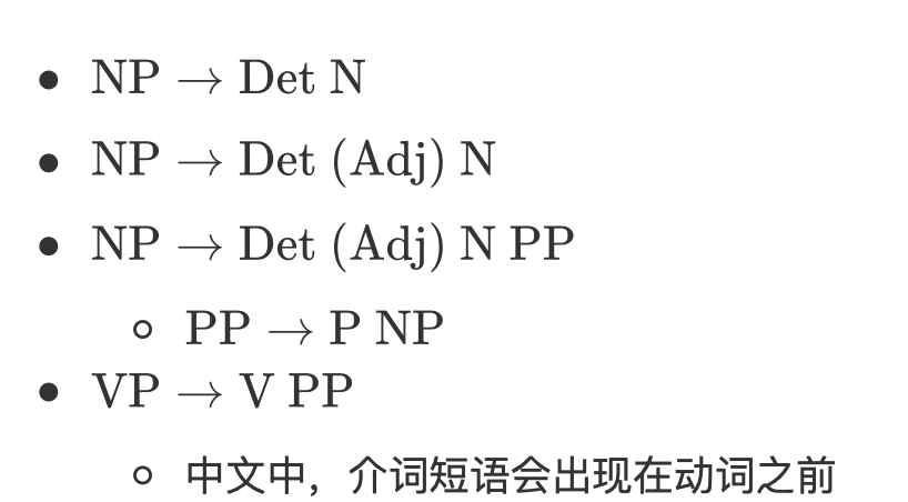
constituency = phrase structure grammer = context-free grammers（CFGs）

• starting unit：word
• words 组合成短语

• 短语可以递归地组合成更长的短语

• Det Determiner限定词

• NP Noun Phrase名词短语
• VP Verb Phrase动词短语
• P Preposition 介词
  • PP Prepositional Phrase介词短语

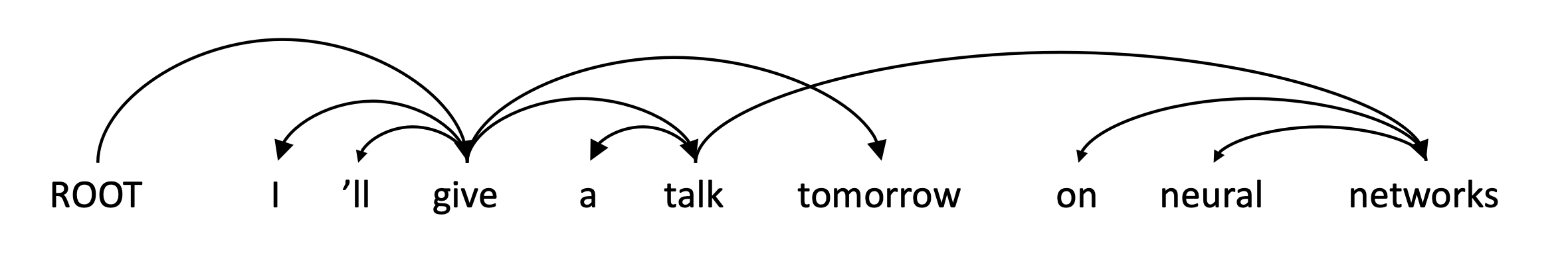
dependency structure

用单词间的依赖/修饰关系表示句子的结构

why do we need sentense structure

• 自然语言中将单词组合成更大的短语、句子来表达复杂的含义和思想
• 人类在理解自然语言是需要弄清楚单词间的相关性
• 自然语言模型需要同样的、理解句子结构的能力

some ambiguity

PP attachment ambiguity 介词短语歧义

• San Jose cops kill man with knife

  • San Jose cops kill man with knife
    • knife是man的modifier
  • San Jose cops kill man with knife
    • knife是kill的modifier

• 关键是如何分析依存关系

  • 对复杂的句子结构，有指数级的依存关系parsing tree
  • Catalan number $C_n=(2n)!/[(n+1)!n!]$
    出现在树形结构的环境中，如n+2多边形的三角剖分可能数

coordination scope ambiguity 协调范围模糊

• Shuttle veteran and longtime NASA executive Fred Gregory appointed to board
  • Shuttle veteran and longtime NASA executive Fred Gregory appointed to board
    • shuttle veteran 和 longtime NASA executive 都是指Fred
  • Shuttle veteran and longtime NASA executive Fred Gregory appointed to board
    • 仅longtime NASA executive 是指Fred

adj adv modifier ambiguity

• Students get first hand job experience
  • Students get first hand job experience
    • first hand 修饰 job
  • Students get first hand job experience
    • first hand 修饰 experience

VP attachment ambiguity

• Multilated body washed up on Rio beach to be used for Olympics beach volleyball
  • Multilated body washed up on Rio beach to be used for Olympics beach volleyball
    • to be used 修饰 body
  • Multilated body washed up on Rio beach to be used for Olympics beach volleyball
    • to be used 修饰 beach

dependency grammar and dependency structure

dependency syntax中单词间的关系通常是二元不对称的依赖关系（箭头 ）

• 箭头连接head和dependency
  • head->dependency
• 依赖关系形成单头无环的图
• 通常额外引入一个ROOT节点，使所有单词有head

universal dependency treebanks

统一、并行、通用的依赖关系描述

• 人工编写语法规则，训练得到parser
• 规则愈发复杂，不能重用之前的工作

treebank

• 起初构建treebank比语法规则要慢且用处有限
• 可重用
  • 在treebank基础上建立parser、tagger等
  • 语言学的
• 覆盖面广泛
• 利用了统计信息
• 可以评估NLP系统

dependency conditioning preference

依赖解析的信息：

• Bilexical affinities两个单词间的密切关系
• Dependency distance：大多数依赖都是和相邻词的
• intervening material：依赖关系很少跨越中间动词or标点符号
• valency of head：不同类型head的依赖关系位置相对固定

Dependency Parsing

• 为每个单词选择其dependency来解析句子
• 只有一个单词是依赖于root的
• 不能成环（只能成tree）
• 箭头可以交叉，不交叉的称为non-projective

projectivity

• 单词按线性顺序排列时，没有交叉的dependency。
• CFG树的依赖关系必须是projective的
• non-projective结构解释移位的word

介词搁浅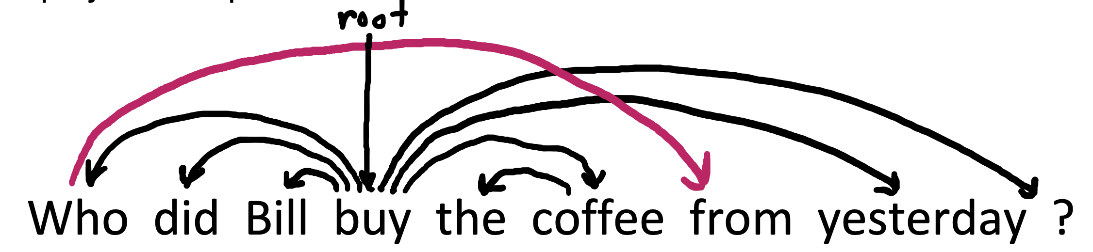

methods

• Dynamic programming
  • Eisner提出的复杂度为$O(n^3)$的clever algo，通过在末尾而非中间生成head
• Graph algo
  • 对句子建立最小生成树（Minimun Spanning Tree）
• constraint satisfaction
  • 去掉不满足硬约束的edge
• transition-based parsing or deterministic dependency parsing
  • 基于ml classifier的贪心选择
  • 比较复杂，具体详见本课程Lecture4

Lecture 5. Recurrent Neural Networks and Language Models

---

how do we gain from a neural dependency parser

• indicator feature 的问题：

  • 这样的特征向量很稀疏
  • 特征不完整
  • 特征的计算开销很大

• distributed representation

  • 将每个单词表示为dense vector
  • part-of-sppeech tags和dependency labels也被表示为同样维度的dense vector

• deep learning and non-linear classifier

  • 传统 ML classifer只有linear boundary

graph-based dependency parsers

• 对每个可能的dependency计算score
  • 需要理解单词的contextual representation

more things about NN

regularization

• 完整的loss func包含对所有参数$\theta$的正则化
  • L2 regularization $\lambda\Sigma_k \theta_k^2$
• 正则化可以防止大量特征/深层模型出现过拟合
• 为模型提供了更强的泛化能力（过拟合实际上不是问题，需要泛化能力）

dropout

• 在训练时随机将神经元输出特征的一部分置零（从而不更新该部分权重）
• 避免特征co-adaptation：不会出现某特征仅在其他特征出现时才有用的情况
• 在单层中，可以看做naive bayes（所有权重被独立设置）和logistic regression（权重在所有上下文中设置）的折中
• 可以看做一种model bagging（ensemble model），或是一种特征独立的强正则化

non-linearities

• old：指数级计算
  • logistic（sigmoid）：0～1
  • tanh：1～-1，实际上是重新缩放和移动的sigmoid
    • $tanh(z)=2sigmoid(2z)-1$
• new
  • hard tanh
  • ReLU
    • 神经元要么dead要么就在传递信息
    • 有很好的梯度backflow，训练很快
• varient
  

prameter initialization

• 将权重初始化为小随机值，避免对称性影响学习
• Uniform(-r,r)
• Xavier初始化中，方差和前后层的尺寸有关
  • $Var(W_i)=\frac{2}{n_{in}+n_{out}}$

optimizers

• 简单的SGD很有效
• 其他优化器
  • Adagrad
  • RMSprop
  • Adam（安全有效）
  • SparseAdam

Learning Rate

• lr太大模型会不收敛，太小模型效果会变差
• 在训练时通常需要动态调整lr
  • by hand：k个epoch后减半
  • by formula：$lr=lr_0e_{-kt}$, for epoch t
  • 循环lr

language model and RNN

language modeling

• 语言模型的任务是预测下一位置的单词
  • 给定单词序列$x^{(1)},\dots,x^{(t)}$，计算下一单词$x^{(t+1)}$的概率分布$P(x^{(t+1)}|x^{(t)},\dots,x^{(1 )})$
• 语言模型也可以看做将概率分配给一段text
  • $P(x^{(1)},\dots,x^{(t)})=\Pi^T_{t=1}P(x^{(t)}|x^{(t-1 )},\dots,x^{(1 )})$

n-gram language model

• n-gram：由n个单词组成的块
• 统计不同n-gram出现的频率来预测下一个单词

• Markov假设：

  • $x^{(t+1)}$只取决于之前的n-1个单词
    $\begin{aligned} P(x^{(t+1)}|x^{(t)},\dots,x^{(1 )})&=P(x^{(t+1)}|x^{(t)},\dots,x^{(t-n+2)})\\
    &= \frac{P(x^{(t+1)},\dots,x^{(t-n+2)})}{P(x^{(t)},\dots,x^{(t-n+2)})} \\
    &= \frac{\text{prob of n-gram}}{\text{prob of (n-1)-gram}}\end{aligned}$

• 使用count的统计近似计算以上概率

sparsity problem with n-gram

• 问题：(n-1)-gram + w 的形式不存在，概率为0
  • 解决方案：为每个w设置一个$\delta$的小概率（smoothing）
• 问题：(n-1)-gram的形式不存在，概率为0
  • 解决方案：回退到(n-2)-gram
• n越大，稀疏问题越严重

generating text with n-gram

• 可以生成语法上正确的text，但语义上不连贯。
• 模拟语言的能力需要更大的n，但与sparsity相悖

neural language model

fixed-window neural language model

优点：

• 不存在sparsity问题
• 不需要使用所有n-gram
  问题：
• 窗口太小
• 增大窗口需要增大W（增大模型）
• 输入乘以W中不同的权重，对单词的处理不对称

RNN

• 核心思想：重复使用同样的Weight
  优点：
• 可以处理任意长度的输入
• 理论上可以利用序列之前的信息
• 模型大小不会随输入增大而变化
• 在每个timestep上使用对称的处理方式

问题：

• 时序的递归计算慢
• 长程依赖

training RNN LM

计算每一步的输出概率分布

每一步的损失函数：
$J^{(t)}(\theta)=CE(y^{(t)}, \hat{y}^{(t)})=-\Sigma log\ y_w^{(t)}log\ \hat y_w^{(t)}$

总体损失函数
$J(\theta)=\frac{1}{T}\Sigma\ J^{(t)}(\theta)$

• 在整个corpus$x^{(1)},\dots,x^{(T)}$上计算loss和梯度开销很大，通常对一个sentence和document计算并更新weight

backpropagation for RNN

$W_h$是共享参数，梯度计算：
$\frac{\partial J^{(t)}}{\partial W_h}=\Sigma^t_i\frac{\partial J^{(t)}}{\partial W_h}|_{(i)}$
将各时刻的梯度计算后求和。

以上结论可以通过多变量导数的计算来证明。

backpropagation through time

generating text with a RNN LM

不断采样，采样输出是下一步的输入。

- 比n-gram生成的文本更加流畅，但总体上仍不连贯

• 考虑RNN和手工规则的结合
  • Beam Search

evaluating LM

• 困惑度perplexity
  $\Pi^T_{t=1}(\frac{1}{P_{LM}(x^{(t+1)}|x^{(t)},\dots,x^{(1)})})^{(1/T)}$
• 等于CE-loss的exp

problems with vanishing and exploding gradients

vanishing gradient

• chain rule使反向传播深入后梯度信号越来越小
• proof
  • $h^{(t)} = \sigma(W_hh^{(t-1)}+W_xx^{(t)}+b_!)$
  • 假设$\sigma(x)=x$
  • $\frac{\partial h^{(t)}}{\partial h^{(t-1)}}=diag(\sigma’(W_hh^{(t-1)}+w_x^{(t)}+b_1))W_h=W_h$
  • 那么$\frac{\partial J^{(i)}(\theta)}{\partial h^{(j)}}=\frac{\partial J^{(i)}(\theta)}{\partial h^{(i)}}W_h^{(i-j)}$
  • 如果$W_h$的特征值均小于1(因为使用了线性的$\sigma$所以为1)，则梯度会呈指数衰减；

RNN-LM更善于从顺序上相近的而非语法上相近的单词学习

exploding gradient

$\theta^{new} = \theta^{old} - \alpha \bigtriangledown_\theta J(\theta)$

• 梯度爆炸会让SGD的“步子”过大
• 极端情况下会导致网络中出现inf或NaN

gradient clipping

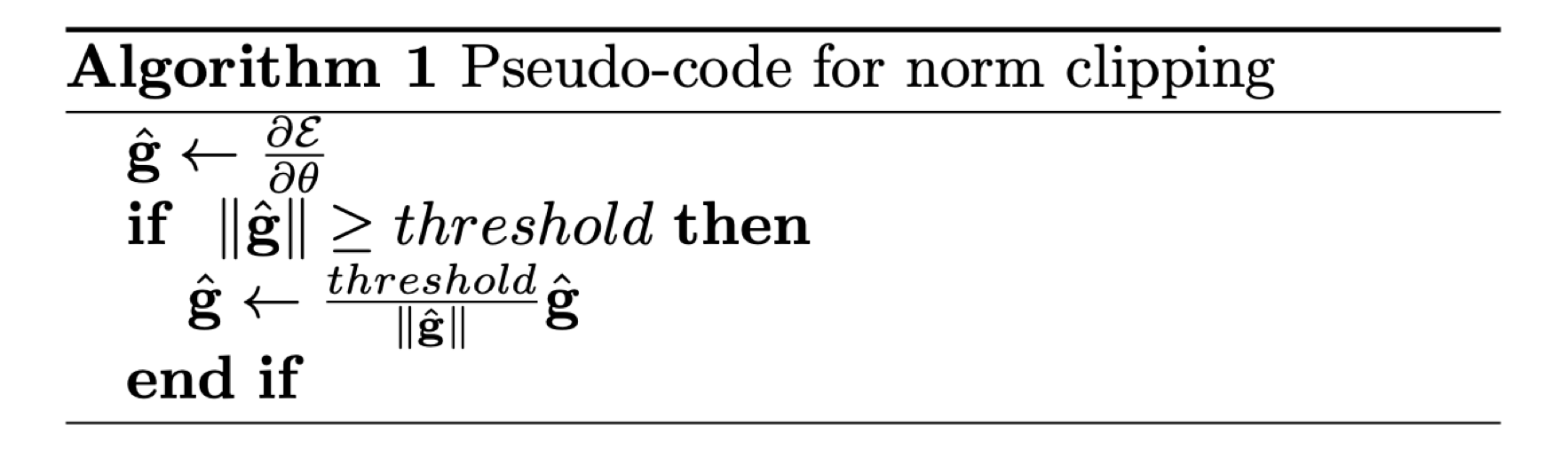
• 在同样的方向上take a smaller step

how to fix the vanishing gradient problem

• RNN中很难学习若干时间步之前的信息
• 使用具有单独记忆的RNN

LSTM

• 在每一步中，拥有两个hidden vector
  • hidden state $h^{(t)}$和cell state $c^{(t)}$
  • 二者都是长度为n的向量
  • cell state保存长期信息
  • LSTM何以从cell读写删信息
• 信息被读/写/删由三个对应的gate控制
  • gates也是长度为n的向量
  • 每一步上，gate的每个元素可以是open 1/close 0/两者之间的一个概率

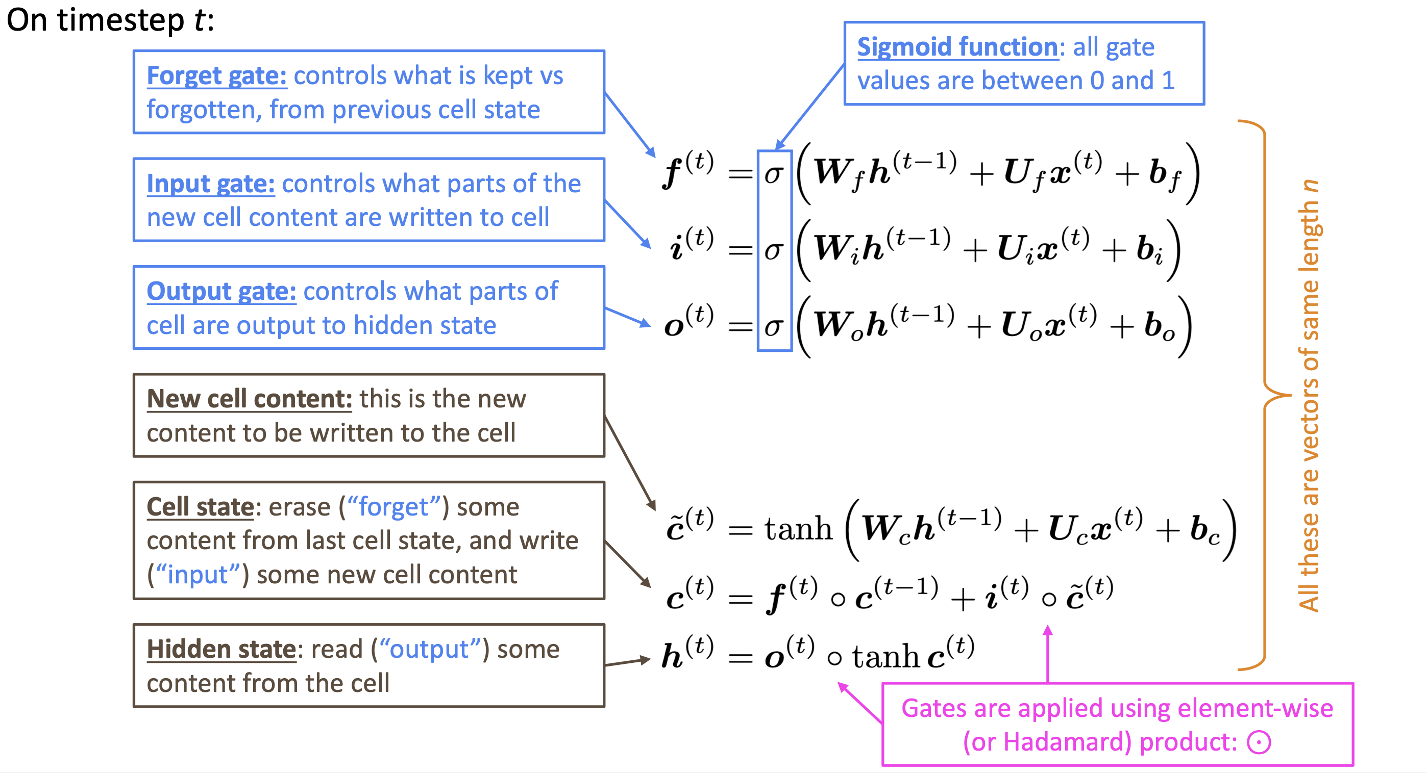
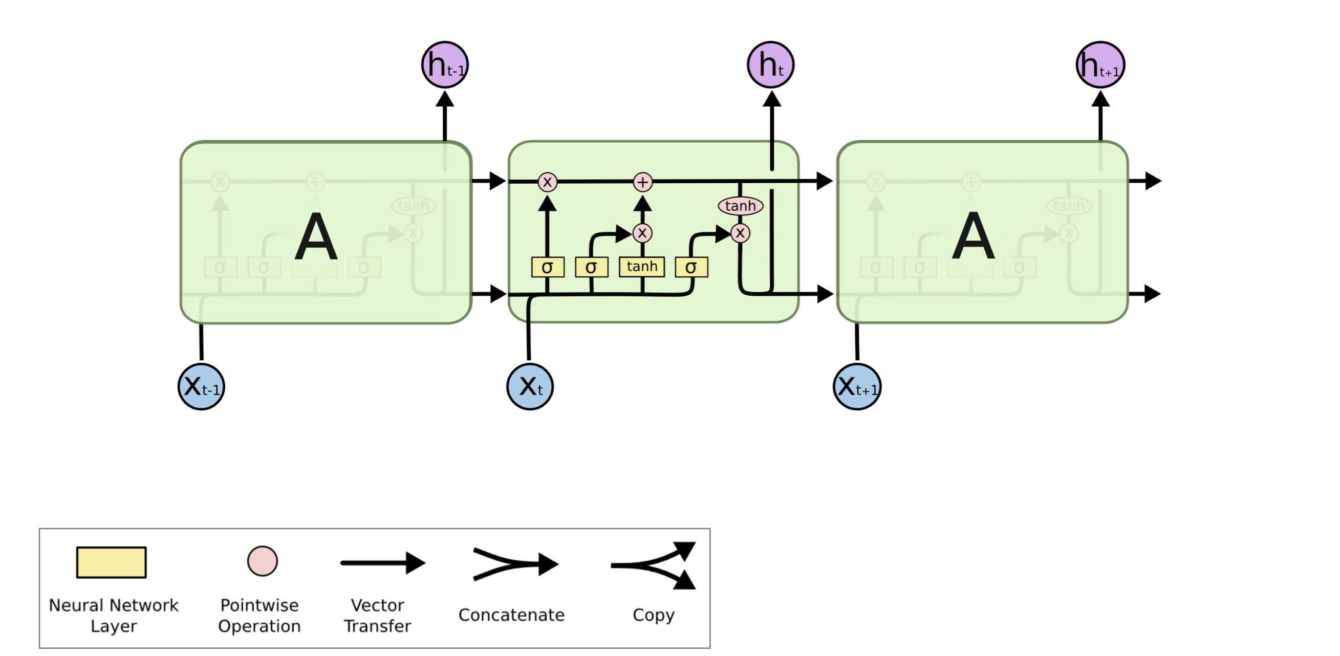
• LSTM相比经典RNN更容易保存时间步上的信息
• 如果forget gate 保存为1，则可以保存所有历史信息
• LSTM的参数也更难学习
• 不保证没有梯度消失和爆炸

is vanishing/exploding gradient just a RNN problem？

• 所有的神经网络结构（尤其是深度解构）都会有
  • chain rule和非线性函数会导致反向传播时梯度很小
  • 低层次的学习很慢
  • RNN中重复乘以统一梯度，更加明显
• solution：添加direct coneection
  • residual connection

bidirectional RNN

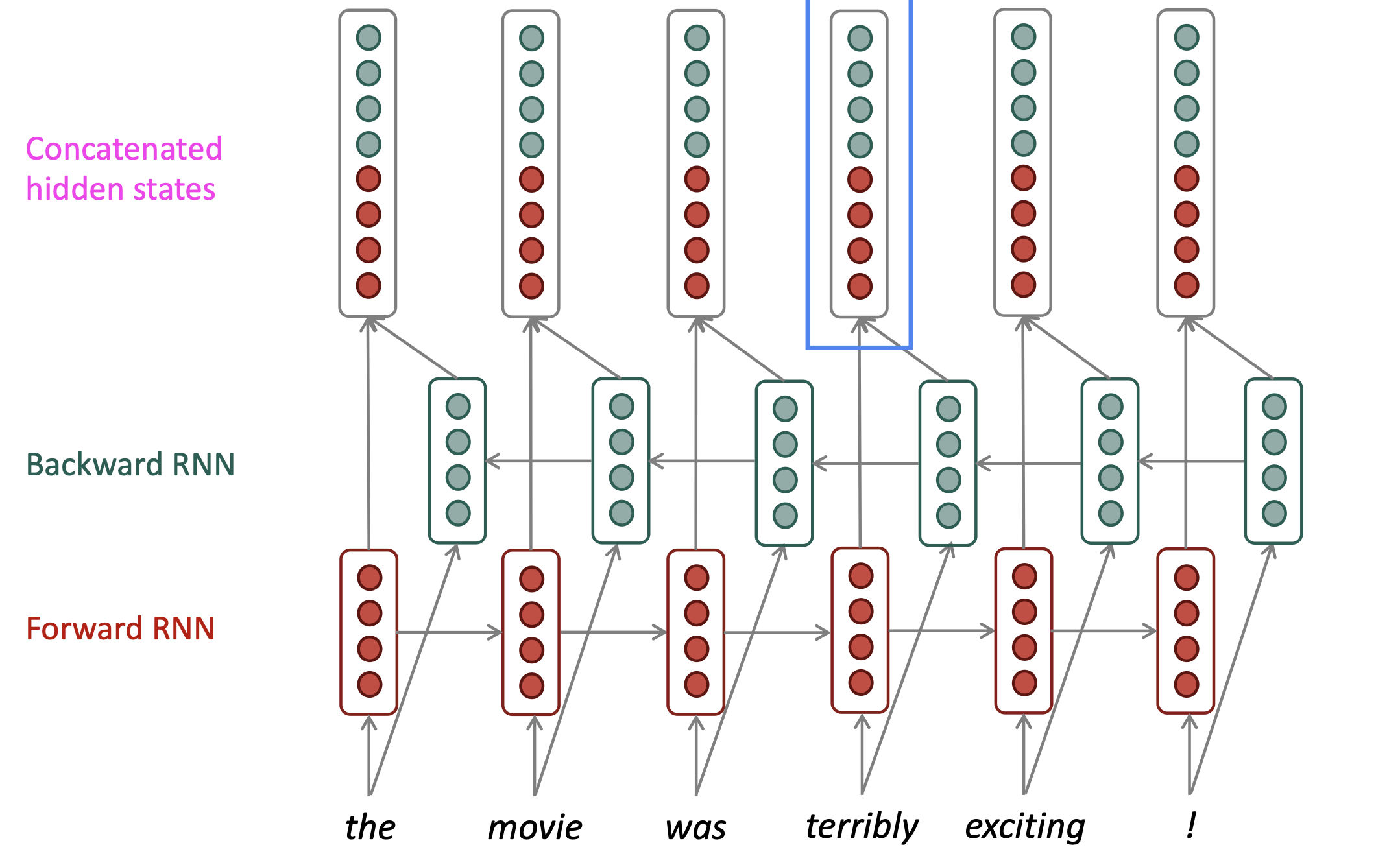
• 包含forward RNN和backward RNN
• 需要有整个输入序列时才能使用（LM中预测下一个word时，相当于只有左边的context，故不能使用双向RNN）

multi-layer RNN

• 堆叠多层RNN，在空间维度上深入（RNN本身是在时序上深入）
• 捕获不同层次的特征
• i层的输入是i-1层的hidden state
• 经验法则：2到4层比较合适

Lecture 7. Machine Translation, Attention, Subword Models

---

machine translation

statistical MT

• 给定法语sentence x，想要找到最好的英语sentence y
• $argmax_xP(y|x)$
• 用bayes rule可以分解为两个组件：$argmax_xP(x|y)P(y)$
• $P(x|y)$
  • 翻译模型，分析单词和短语应该如何翻译
  • 从人工翻译的并行数据中学习
• $P(y)$
  • 语言模型，模型如何生成合适的语言
  • 从单词数据中学习

learning alignment for SMT

• 需要学习$P(x,a|y)$,其中$a$是单词间的对应
• $a$是隐变量，需要用EM算法等来学习

decoding for SMT

• 如何计算argmax，列举所有y并计算概率显然不可行
• 用启发式算法丢弃概率过低的假设

neural MT

sequence-to-sequence model

• encoder+decoder
• 用于很多NLP任务
  • 文本摘要
  • 对话生成
  • 文本解析
  • 代码生成
• 是一种conditional LM
  • $P(y|x)=P(y_1|x)P(y_2|y_1,x)\dots P(y_T|y_1,\dots,y_{T-1},x)$
• sequence-to-sequence是一个端到端的系统，反向传播在整个系统中。

greedy decoding

• 在解码器的每一步都使用argmax（但总体的概率并非最大）
• 无法撤销步骤

exhaustive search decoding

• 计算所有可能的序列，开销很大，有V^T种可能

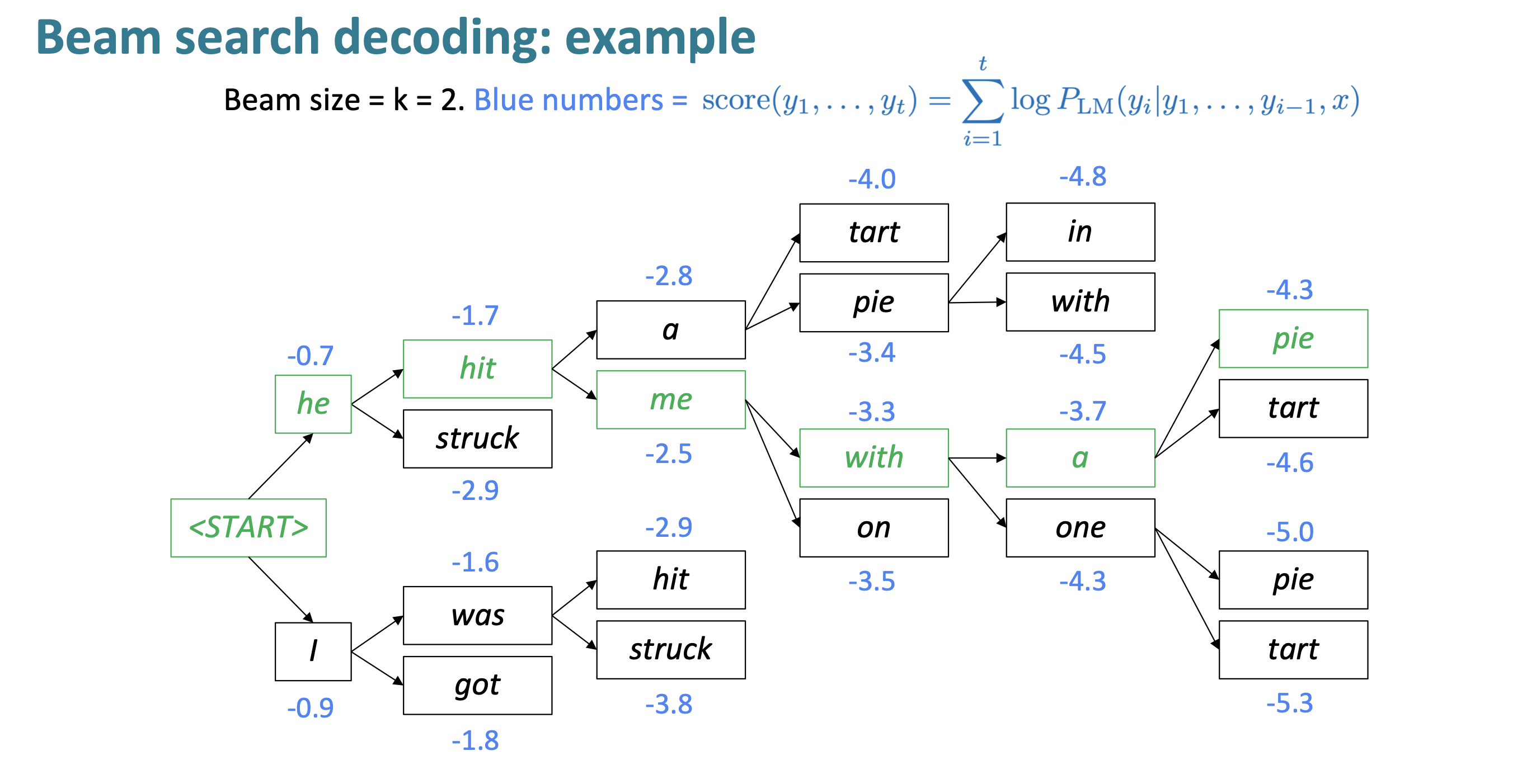
beam search decoding

• 核心思想：在decoder的每一步，跟踪k个最可能的输出（hypotheses）
  • k是beam size，通常为5-10
  • 按得分选择$score=log P_{LM}(y_1,\dots,y_t|x)=\Sigma^t_{i=1}log P_{LM}(y_i|y_1,\dots,y_{i-1},x)$
• 不一定能找到最优解，但效率比穷举高的多

stopping criterion

• 在greedy decoding中会持续解码到$$ token
• 在beem search decoding 中，可能会提前生成$$ token
  • 一个hypothesis到达$$，则其已经完成
  • 继续处理其他hypothesis
• beem search decoding的停止条件：
  • 到达预设timestep T
  • 有预设的n个hypothesis已经完成

finishing up

• 结束时获得了若干个hypothesis，需要从中选择最合适的
• 如果直接使用score，则长度越长score越小
• 需要对score按长度标准化（乘$\frac{1}{T}$）

advantages and disadvantages of NMT

• advantage
  • 性能更好，翻译更通顺，从上下文使用了更多信息
  • 端到端系统
  • 手动工作更少，不需要特征工程和对每种语言单独建模
• disadvantage
  • 可解释性
  • 可控性（无法制定规则）
  • 安全性

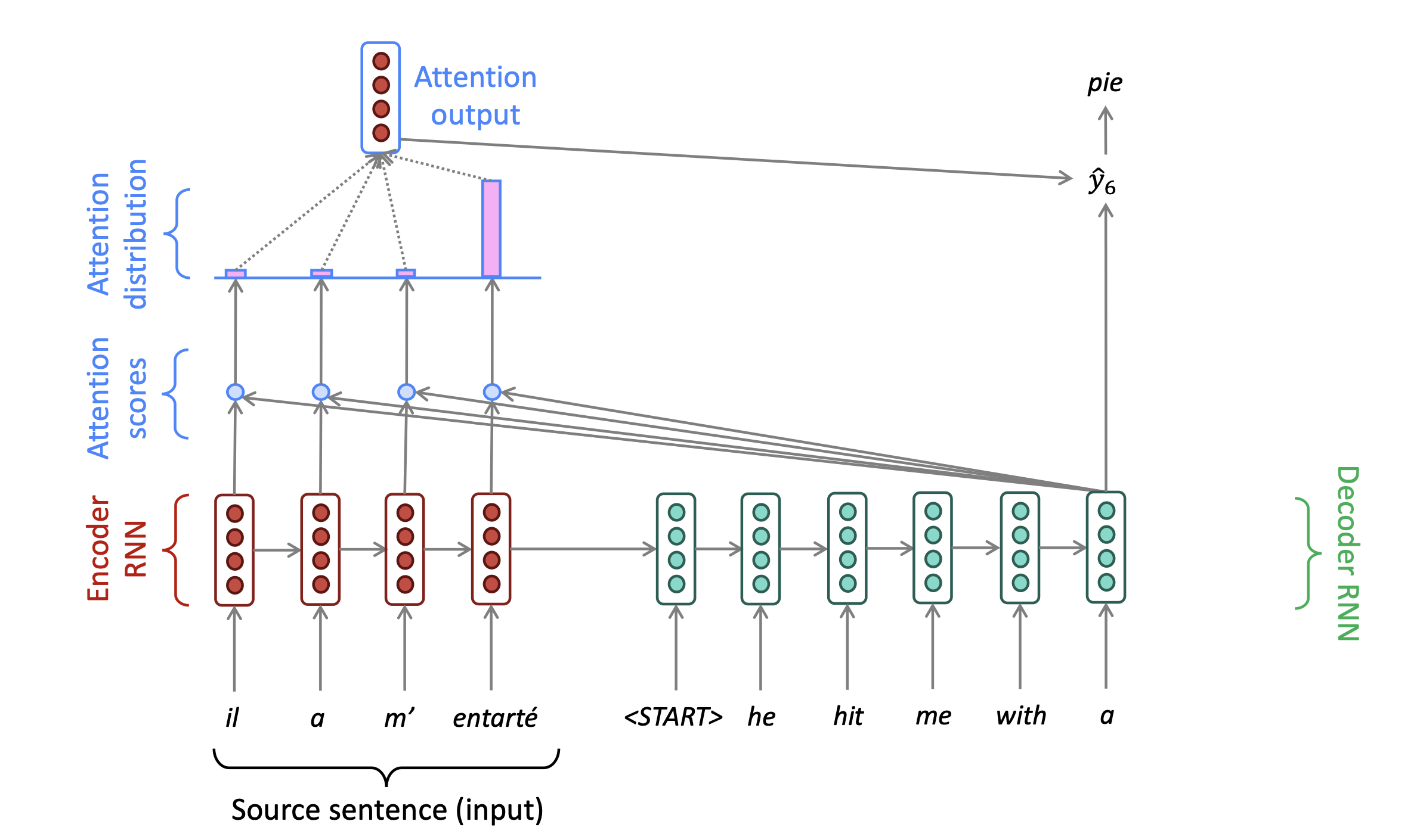
attention

• 源序列encoding过程需要捕获源语句的所有信息，存在信息瓶颈
• attention的核心思想：在decoder的每一步，用encoder的连接来使其能关注到源序列的特定部分

Lecture 8. self-attention and Transformer

---

attention in equations

• encoder hidden states: $h_i\in \mathbb{R}^h$
• decoder hidden state on timestep t: $s_t\in \mathbb{R}^h$
• attention scores: $e^t=[s^T_th_1,\dots,s_t^Th_N]\in\mathbb{R}^N$
• attention distribution: $\alpha^t={\rm softmax}(e^t)\in\mathbb{R}^N$
• attention output $\mathbf{a}_t=\Sigma_{i=1}^N\alpha_i^t\mathbf{h}_i\in\mathbb{R}^h$
• $[\mathbf{a}_t,s_t]\in\mathbb{R}^{2h}$

advantages of attention

• 绕过了信息瓶颈的问题，直接允许decoder连接来自source的信息
• 注意力机制更human-like
• 可以解决梯度消失问题——direct connection
• 可解释性
  • 提供了soft alignment（网络自己学习了alignment）
  • 通过注意力分布可以看到decoder的关注点

attention variants

query attends to the values

给定values $h_!,\dots,h_N\in\mathbb{R}^{d_1}$和query $s\in\mathbb{R}^{d_2}$，attention机制包括：

• 计算attention scores $e\in\mathbb{R}^N$
• 计算softmax获得attention distribution $\alpha={\rm softmax}(e)\in\mathbb{R}^N$
• 对attention distribution加权求和 $\mathbf{a}=\Sigma_{i=1}^N\alpha_i\mathbf{h}_i\in\mathbb{R}^{d_1}$

几种attention方法

• dot-product attention: $e_i=s^Th_i$
  • 要求$s$和$h$维度相同
• multiplicative attention: $e_i=s^TWH_i$
  • $W\in\mathbb{R}^{d_1\times d_2}$是一个额外的权重矩阵
  • 权重似乎过多，需要学习对所有部分的attention
• reduced rank multiplicative attention: $e_i=s^T(U^TV)H_i=(Us)^T(Vh_i)$
  • $I\in\mathbb{R}^{k\times d_2}, V\in\mathbb{R}^{k\times d_1},k\ll d_1,d_2$
• additive attention: $e_i=v^T{\rm tanh}(W_1h_i+W_2s)$
  • $W_1\in\mathbb{R}^{d_3\times d_1},W_2\in\mathbb{R}^{d_3\times d_2}$是权重矩阵，$v\in\mathbb{R}^{d_3}$是权重向量
  • 实际上用了一个网络来计算attention

Lecture 9. Transformers

---

Transformer

Issues with RNN

• Linear interaction distance：捕获两个词的交互需要$O(sequence length)$ steps
  • 长程依赖问题（梯度难以传播）
  • 线性顺序的输入处理sentence不合理
• Lack of parallelizability
  • forward 和 backward都需要$O(sequence length)$

if not recurrence, the what?

• word window(CNN)
  • 1D-Conv
  • maximum interaction distance = sequence length/window size——通过多层卷积
• attention

self-attention

self-attention equation

• query $q_i\in\mathbb{R}^d$
• key $k_i\in\mathbb{R}^d$
• value $v_i\in\mathbb{R}^d$
• 对self-attention来说，q,k,v来自同一个东西
  • 最简单的方式是$q_i=k_i=v_i=x_i$
  • 此时$e_{ij}=q_i^Tk_j$
  • $\alpha_{ij}=\frac{exp(e_{ij})}{\Sigma_{j’}exp(e_{ij’})}$
  • $output=\Sigma_j{\alpha_{ij}v_j}$

Problem1. sequence order(position embedding)

• self-attention对语序完全不敏感，所以需要编码order
• 考虑将sequence index编码为vector $p_i$，加到qkv上

sinusoidal position representations

$PE_{(pos,2i)}=sin(pos/10000^{2i/d_{model}})$
$PE_{(pos,2i+1)}=cos(pos/10000^{2i/d_{model}})$

• 绝对位置并不那么重要
• 可以外推到更长的长度（周期性）
• 没有可学习的参数

learned absolute position representation

学习position embedding matrix $p \in \mathbb{R}^{d\times T}$

• 比较灵活，每个位置都可以根据data去学习
• 长度固定，无法外推

Problem2. lack of nonlinearities

• self-attention只是weighted average，不包含非线性
• 解决方案
  • 添加一个feed-forward network对输出做后处理
  • $m_i=MLP(o_i)=W_2ReLu(W_1o_i+b_1)+b_2$

Problem3. “don’t look at the feature”

• 在decoder中需要mask
• mask out attention to future words——将attention scores设置为$-\infty$

Transformer

key-query-value attention

• $k_i=Kx_i, K \in\mathbb{R}^{d\times d}\text{ is the key matrix}$
• $q_i=Qx_i, Q \in\mathbb{R}^{d\times d}\text{ is the query matrix}$
• $v_i=Vx_i, V \in\mathbb{R}^{d\times d}\text{ is the value matrix}$
• $output=softmax(XQK^TX^T)XV$

multi-head attention

• $Q_l,K_l,V_l\in \mathbb{R}^{d\times\frac{d}{h}}$
• 计算attention然后concat

Residual connection

• instead of $X^{(i)}=Layer(X^{(i-1)})$
• let $X^{(i)}=X^{(i-1)+Layer(X^{(i-1)})$

layer normalization

• layernorm的成功可能因为其对梯度的norm
• $x\in\mathbb{R}^d$是一个单独的word vector
• $\mu=\Sigma_{j=1}^dx_j\in \mathbb{R}$是均值
• $\sigma=\sqrt{\frac{1}{d}\Sigma_{j=1}^d(x_j-\mu)^2}\in\mathbb{R}$是标准差
• $\gamma\in\mathbb{R}^d,\beta\in\mathbb{R}^d$是可学习的gain和bias参数(工业上的习惯)
• $output=\frac{x-\mu}{\sigma+\epsilon}*\gamma+\beta$

scaled dot-product

• 向量维度很大时，dot-product也会很大，导致softmax很陡峭，梯度很小
• ${\rm Attention}(Q,K,V)={\rm softmax}(\frac{QK_T}{\sqrt{d_k}})V$

why fix about Transformer

• quadratic compute in self attention
  • linear in RNN
• position representation
  • relative linear position attention
  • dependency syntax-based position

varient of Transformer

• for quadratic compute
  • 投影到更低维度计算attention （linformer）
  • 不计算所有的pairs，只计算一部分（BigBird）

for pretrain

• 如果只用decoder，则不需要cross attention和layernorm

Lecture 10. Transformers and pretrain

---

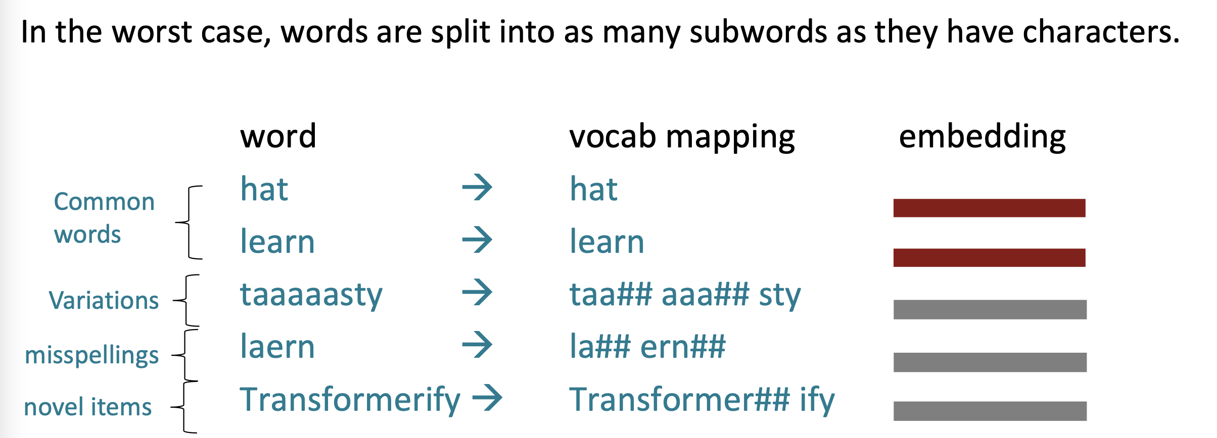
word structure and subword models

• 测试时遇到的OOV word将会被映射为UNK
• 有限的词汇显然不能满足很多语境

the byte-pair encoding algorithm

• 从只包含单个字母的vocabulary开始
• 寻找最常相邻出现的字母，将其添加为subword
• 不断添加直到特定的大小

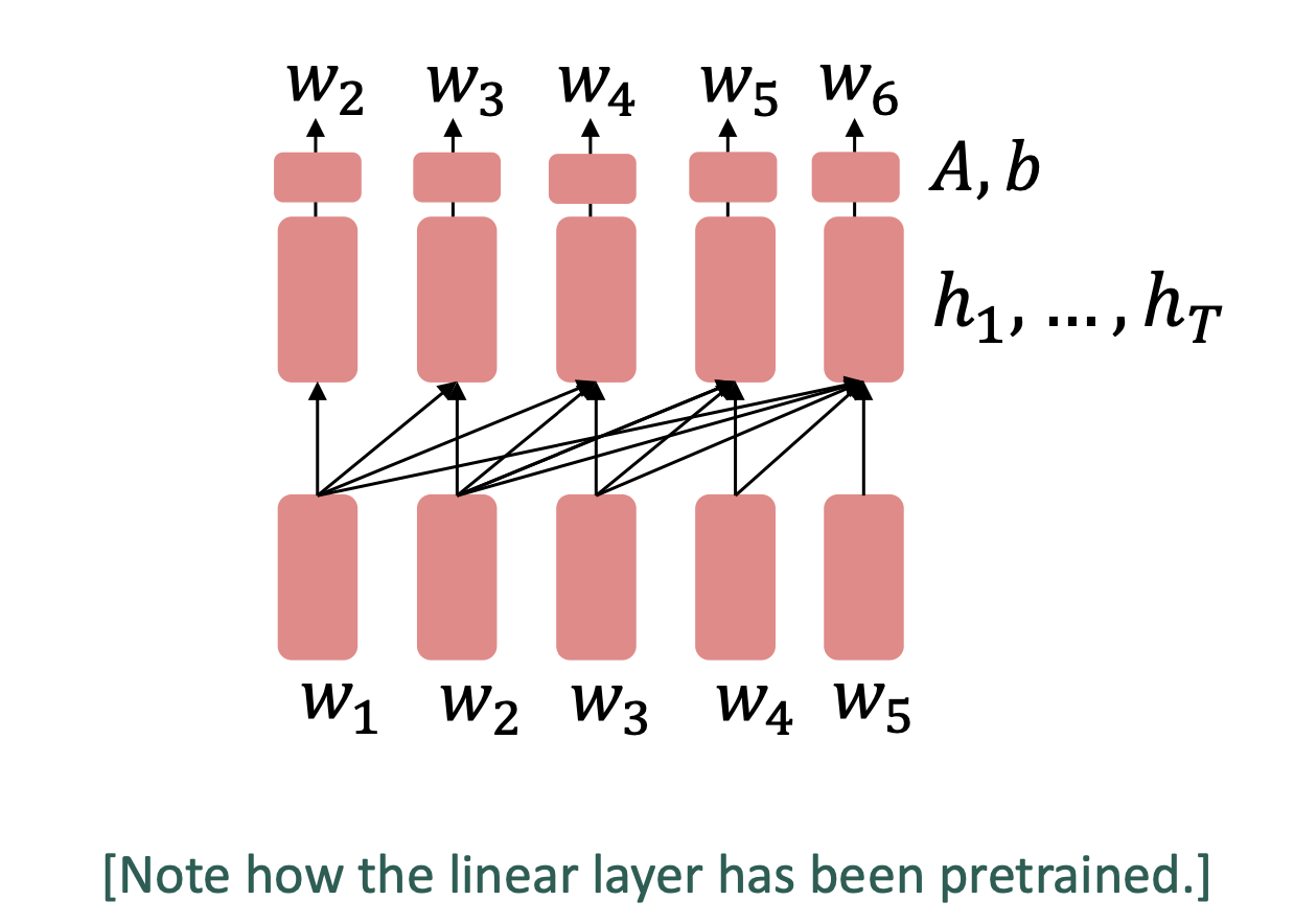
Motivating model pretraining from word embedding

two types of pretrain

pretrained word embedding

• 仅预训练词向量
• 预训练的训练数据必须能够充分学习上下文
  • 一个word的预训练词向量是固定的，与上下文无关
• 整个网络的大部分仍是随机初始化的

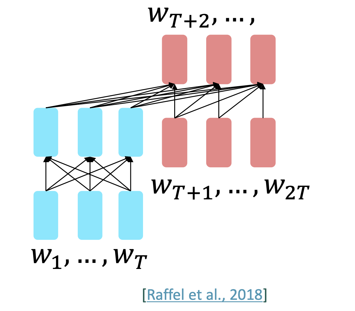
pretraining whole models

• 所有参数都被pretrain
• 可以学习语言的概率分布

three ways of model pretrain

• decoder
  • LM
  • 生成任务，看不到future word
• encoder
  • 有双向的context
  • 如何训练？？
• encoder-decoder

Decoder

• finetune可以忽略pretrained model原本的任务
  

• 可以继续用generator的方法(Prompt)
  

• GPT

  • 12层 Transformer decoder
• GPT-2
  • 更大的GPT

Encoder

• encoder方法中可以看到双向的上下文，不能直接用LM方法训练

• Idea：用[MASK] token盖住部分word，让模型预测被盖住的word

  • 只添加masked word 的loss，称作Masked LM

• BERT

  • 预测15%的(sub)word
    • 80% 用[mask]替换
    • 10% 用随机的token替换
    • 10% 不变（但仍然predict）
  • bert也预测下一个chunk是真实follow的还是随机采样的，即next sentence prediction（NSP）

limitation of pretrained encoders

• 在生成任务上最好使用decoder
• bert在自回归任务上并没有那么好

extension of bert

• RoBERTa：train BERT for longer and remove next sentence prediction
• SpanBERT：连续mask——更难且有用的任务

encoder-decoder

• Encoder编码prefix且不进行预测，Decoder预测后面的部分

• encoder从context受益，decoder则像LM一样预测

• T5
  

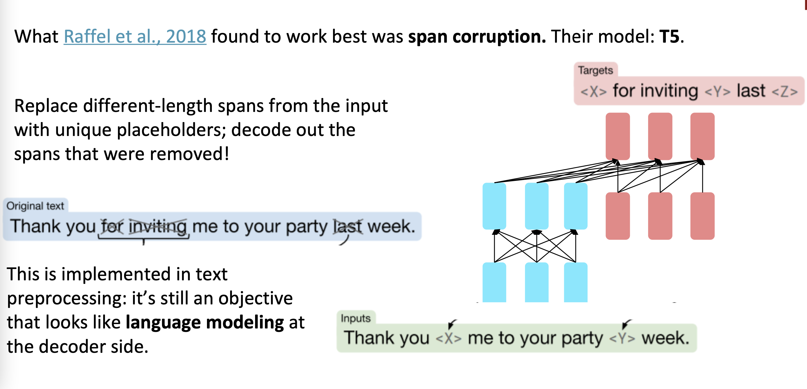
  • span corruption
    • 从输入中用特定的占位符去替代不同长度的文本（和BERT不同的是，T5只知道此处缺失，不知道缺失的长度）
    • decoder解码出缺失部分

very large model and in-context learning

• 两种使用pretrained model的方式：
  • prompt
  • finetune
• GPT-3
  • seems to perform some kind of learning withou gradient steps simply from examples you provide within their contexts
  • in-context learning：甚至没有finetune

Lecture 11. QA (Chen Danqi)

---

QA

Read Comprehension

• 理解一段text，然后回答一段问题 $(Passage, Question)->Answer$

• Problem formulation for SQuAD(Stanford的QA数据集，answer在passage中出现)

  • Input: $C=(c_1,c_2,\dots,c_N),Q=(q_1,q_2,\dots,q_M),c_i,q_i\in V$
  • Output: $1\le start \le end le N$

• neural models for reading comprehension

  • LSTM-based model
  • BERT finetune model

LSTM-based model

• MT任务中的source和target变成passge和question
• 需要通过attention建模哪些word和question最相关，以及和question中哪部分word相关
• 不需要auto regressive decoder，而是训练预测start和end位置的分类器

BiDAF(Bidirectional Attention Flow)

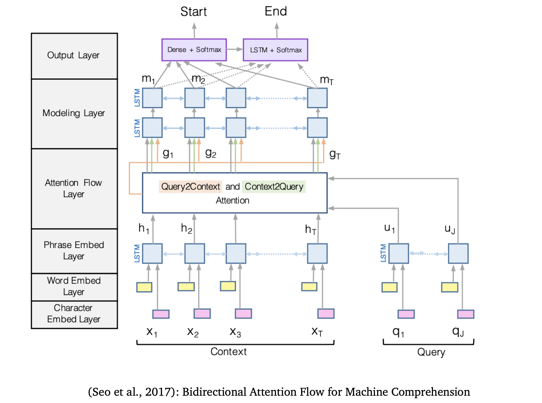
• Encoding：character embed layer+word embed layer+phrase embed layer
  • $e(c_i)=f([Glove(c_i);charEmb(c_i)])$
    $e(q_i)=f([Glove(q_i);charEmb(q_i)])$
    将word embedding（GloVe）和character embedding（CNN+maxpooling over character embedding）拼接在一起，并通过high-way networks
  • 用Bi-LSTM生成context和query的上下文embedding
• attention：attention flow layer
  • context-to-query attention：对context中的word，寻找query中与之最相关的word
  • query-to-context attention
  • 计算每个词对的similarity score
    $S_{i,j}=w_{sim}^T[c_i;q_j;c_i\odot q_j]\in\mathbb{R}, w_{sim}\in\mathbb{R}^{6H}$
    c2q: 找出和c_i相关的question words $\alpha_{i,j}=softmax_j(S_{i,j})\in\mathbb{R}, a_i=\Sigma_j\alpha_{i,j}q_j\in\mathbb{R}^{2H}$
    q2c: 找出context中重要的词 $\beta_i=softmax_i(max_j(S_{i,j}))\in\mathbb{R}^{N}, b_i=\Sigma_i\beta_ic_i\in\mathbb{R}^{2H}$
    output: $g_i=[c_i;a_i;c_i\odot a_i;ci\odot b_i]\in\mathbb{R}^{8H}$
• modeling and output layer
  • modeling layer： 将$g_i$送进两层Bi-LSTM
    $m_i=BiLSTM(G_i)\in\mathbb{R}^{2H}$
    • attention layer用于建模query和context的关系
    • modeling layer用于建模 context内部的关系
  • output layer： 两个用于预测start和end位置的classifer
    $p_{start}=softmax(w_s^T[g_i;m_i])$
    $p_{end}=softmax(w_e^T[g_i;m_i’]), m_i’=BiLSTM(m_i)\in\mathbb{R}^{2H}$

Bert for reading comprehension

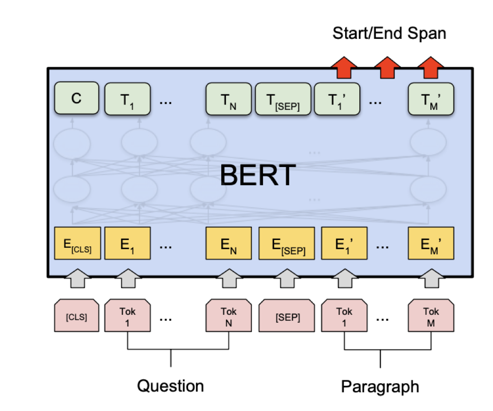
comparisons

• BiDAF等模型捕获question和passage的关系
• BERT在question和passage的concat上做self-attention（attention(p,q),attention(q,p),attention(p,p),attention(q,q)），包含了q和p的关系
• Clark and Gardner, 2018证明在BiDAF中添加attention(p,p)可以获得提升

Lecture 12.natural language generation（Antoine Bosselut）

---

natural language generation（Antoine Bosselut）

what is NLG

• NLG task
  • Machine Translation
  • dialogue systems
  • Summarization
  • Data-to-Text Generation
  • visual description
  • creative generation

formulating for NLG

• auto-regressive model
• Step： $S=f({y_{<t},\theta})$
  $P(y_t|{y_{<t}})=\frac{exp(S_w)}{\Sigma_{w’\in V}exp(S_{w’})}$
• Loss: $L=-\Sigma_t logP(y_t|{y_{<t}})$

decoding from NLG models

Greedy methods

• argmax decoding
• beam search

get random: sampling

top-k

• 每次只选top k个token
• 增大k会让模型更多样也容易出错
• 减小k会让模型更greedy

top-p

• top-k的问题
  • 对平滑的分布，top-k会削减许多可能的选项
  • 对陡峭的分布，top-k会添加许多不太可能的选项
• solution
  • 根据分布的特点，动态选取k
  • 调整（rebalance）概率分布：除以一个超参数 $\tau$后再计算softmax

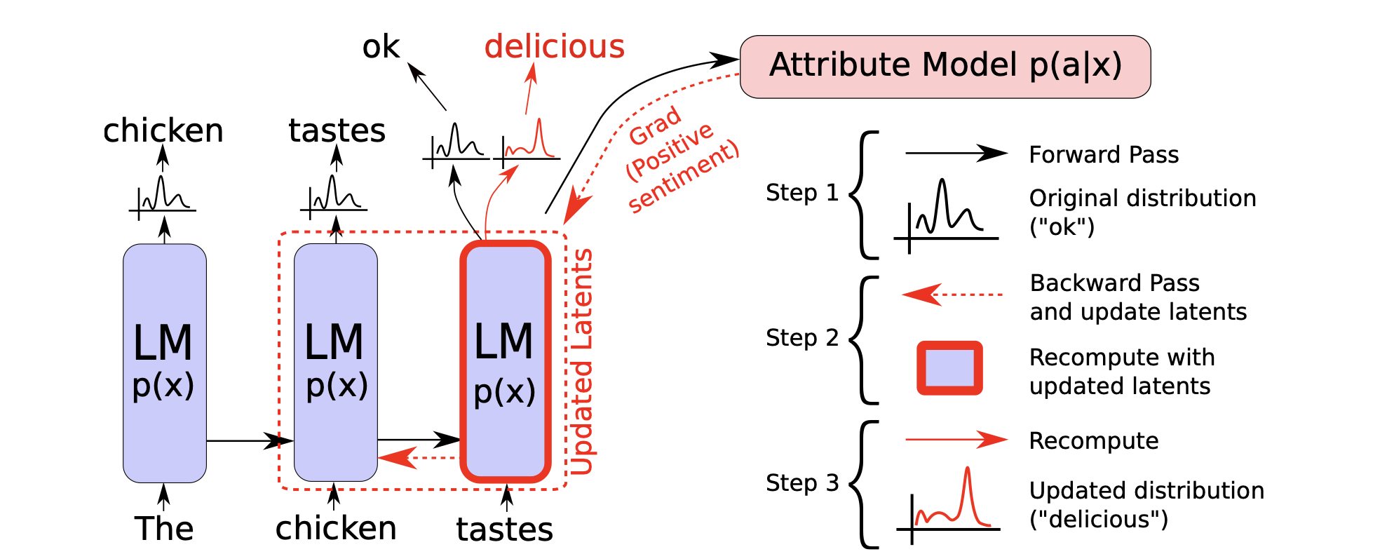
re-balancing distribution

仅依赖model输出的概率分布可能并不可靠

• 根据n-gram的统计数据来调整概率分布
• 根据梯度反向传播调整概率分布
  

traning NLG models

Maximum Likelihood Training

$L=-\Sigma_t logP(y_t|{y_{<t}})$

不利于多样化的text generation

Unlikelihood Training

给定一个不期望得到的token 集合$\mathcal{C}$，降低其在上下文中的likelihood

$\mathcal{L}_{UL}^t=-\Sigma_{y_{neg}\in\mathcal{C}}log(1-P(y_{neg}|\{y\}_{<t}))$

将unlikelihood和likelihood结合
$\mathcal{L}_{ULE}=\mathcal{L}_{MLE}+\alpha\mathcal{L}_{UL}$

exposure bias问题

• 训练时，模型输入的是gold context；生成时，模型输入是decoder之前的输出
• Solution
  • scheduled sampling
    • 以概率p解码出一个token并送入模型作为下一个input（而非gold token）
    • 在训练过程中逐渐增大p
    • 但训练中同时也会生成一些奇怪的输出
• dataset aggregation
  • 在训练过程中，生成一些新序列加入训练集
• sequence re-writing
  • 在corpus中搜索一个human-written的prototype text，
• reinforcement learning

evaluating NLG

• N-gram overlap metrics——BLEU、ROUGE、METEOR（效果不好）
• semantic overlap metrics——PYRAMID、SPICE、SPIDEr
• model-based metrics
  • word distance functions
    • vector similarity
    • word mover’s distance
    • bert score
  • beyond word matching
    • sentnce movers similarity
    • BLEURT
• human evalutions

Lecture 13. Coreference resolution

---

Co-reference resolution

what is co-reference resolution

• 识别出文本中共指同一个实体的单词

• application

  • 文本理解
    • 信息抽取、QA、summarization
  • 机器翻译
  • 对话系统

co-reference resolution in two steps

• detect the mentions——easy
• cluster the mentions——hard

mention detection

• detect a span of text referring to some entity
  • pronouns: I, your, it, she, him, etc.
  • named entitied: people, place, Biden, etc.
  • noun phrase: a dog, etc.
• 简单但没那么简单
  • 很多结果并非mentions
  • it is sunny、every student

how to deal with bad mentions

• 可以训练一个分类器来过滤掉spurious mentions
  • POS tagger、NER、parser
• 更常用的方法：让所有的mentions都作为”candidate mentions”
  • 在co-reference 系统运行完后，丢弃掉这些mention

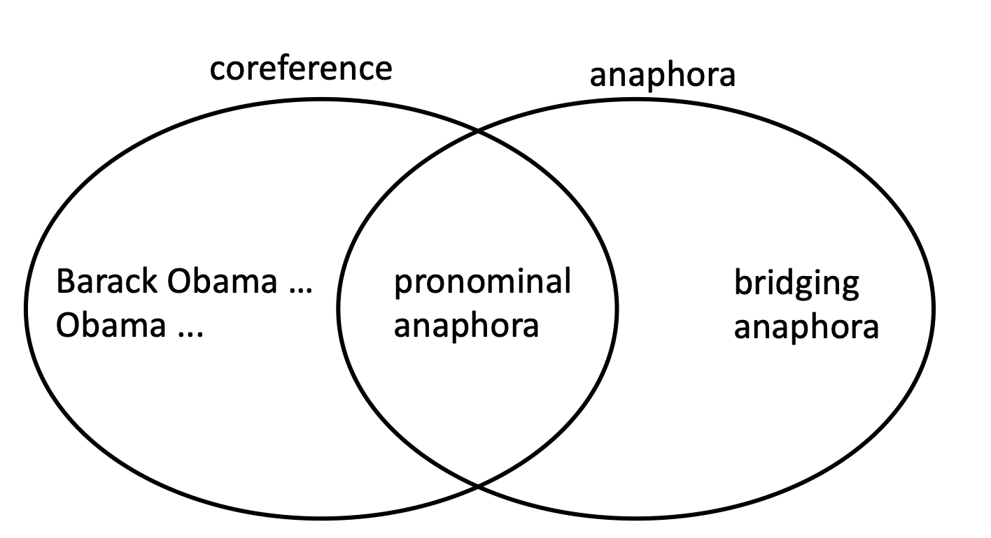
some linguistics

• co-reference：两个mention指代同一个实体

• anaphora：一个照应词anaphor指代另一个先行词antecedent

• 并非所有的anaphoric关系都是co-referential

  • 并非所有的词都有reference
    • every dancer twisted her knee
      二者都有
    • no dancer twisted her knee
      存在anaphoric但没有co-referential
  • bridging anaphora
    • We went to see a concert last night. The tickets were really expensive.
    • tickets对concert没有co-reference，是bridging anaphora的关系

4 kinds of co-reference models

• Rule-based（pronominal anaphora resolution）
• mention pair
• mention ranking
• clustering

Hobbs’ naive algo

• Rule-based

• 并未真正理解语言

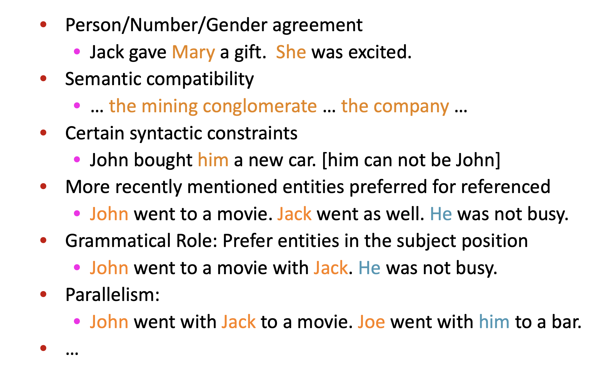
• Knowledge-based Pronominal Coreference

  • She poured water from the pitcher into the cup until it was full.
  • She poured water from the pitcher into the cup until it was empty.
  • The city council refused the women a permit because they feared violence.
  • The city council refused the women a permit because they advocated violence

mention pair

• 训练一个二分类器，对每个mention pair分类
• Loss：regular CE loss
  • $J=-\Sigma^N_{i=2}\Sigma^i_{j=1}y_{ij}log\ p(m_j,m_i)$

• 选择一定的阈值，置信度大于该阈值即添加co-reference 连接

• disadvantage

  • 许多mention只有一个co-reference 连接
• solution
  • 对每个mention只计算一个antecedent

mention ranking

• 为得分/概率最高的candidate添加连接
• Loss：
  • $J=\Sigma^{i-1}_{j=1}\mathbb{1}(y_{ij}=1) p(m_j,m_i)$$

how to calculate score/probability

• Non-neural statistical classifier
• Simple neural network
• More advanced model using LSTMs, attention, transformers

Non-Neural model: Features

neural model：标准前馈神经网络

• 输入word embedding和distance、document genre体裁、speaker infomation等其他特征

neural model：CNN

• 忽略了语法信息，并不那么linguistically

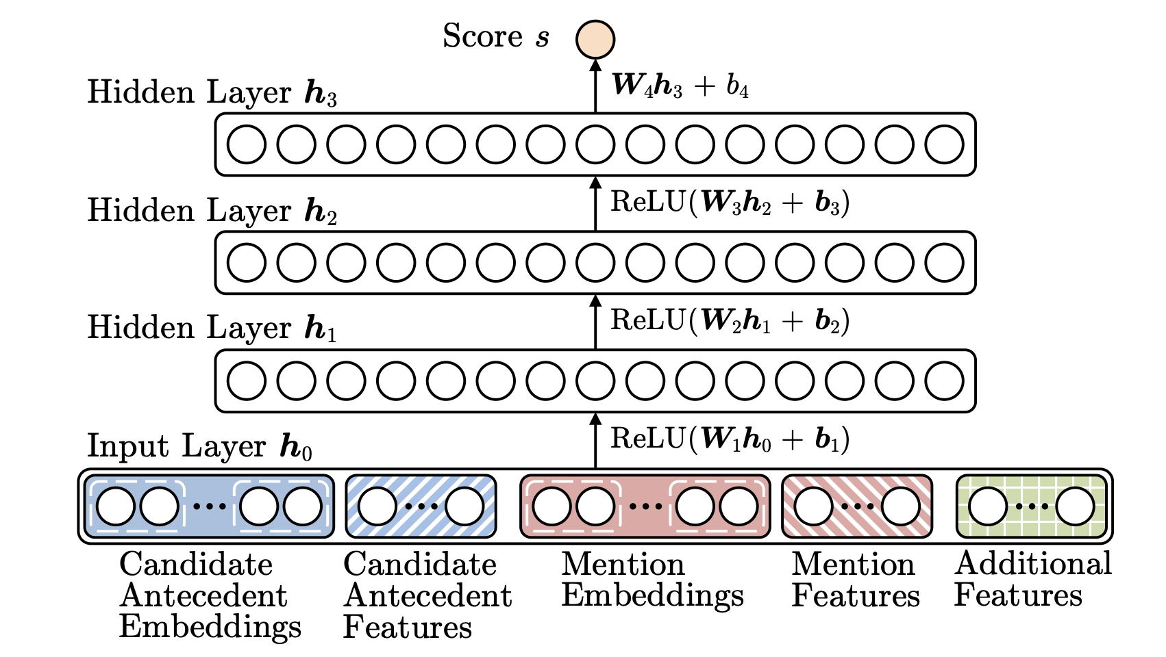
neural model：end-to-end neural coref model

• mention ranking model
• 在FFN基础上使用LSTM、attention
• 没有mention detection的过程
• 不再将每段文本都作为candidate，利用attention去修剪

模型架构：

• 用character-level CNN embed the words
• 将document送入Bi-LSTM
• 将每个span表示为向量
• 计算每对span的得分

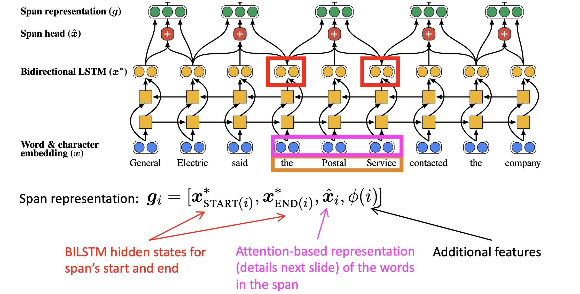
$\hat x_i$是span中word embedding的attention加权求和。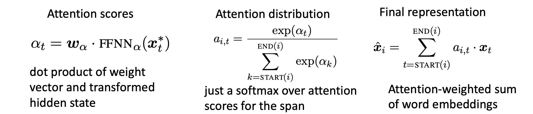

• $score(i,j)=s_m(i)+s_m(j)+s_a(i,j)$
• $s_m(i)=w_m\cdot FFNN_m(g_i)$ 表征i是否为mention
• $s_a(i,j)=w_a\cdot FFNN_a([g_i,g_j,g_i\circ g_i,\phi(i,j)])$表征i和j是否coreferent

neural model：BERT-based model

• idea
  • 预训练在span-based预测任务上（coref和QA）表现更好的BERT模型
  • BERT-QA：将coref看作QA task
    • Q：mention
    • A：mention的antecedent

co-reference evaluation

• B-cubed
  • 对每个mention计算p和r
  • 对P和R取平均

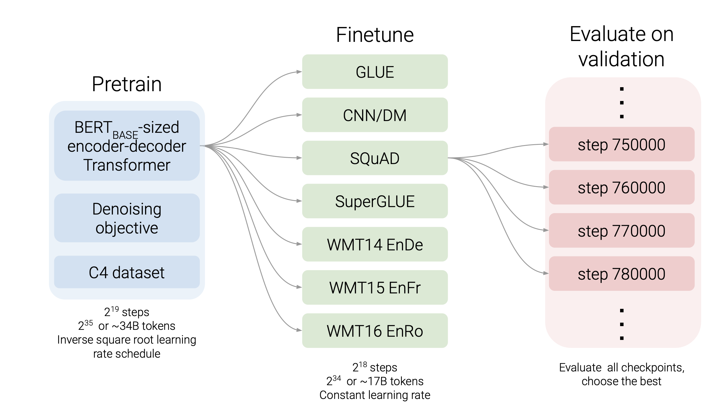
Lecture14. T5 and large LM:the good, the bad and the ugly(Colin Raffel)

---

T5 and large LM

larger LM

• larger corpus
• more parameters
• more tokens
• different optimizer

T5(Text-to-text Transfer Transformer)

• text-to-text task
  • MT
  • CoLA(Corpus of Linguistic Acceptability)
  • STS-B(Semantic Textual Similarity Benchmark)
  • summarize
• pre-train dataset
  • C4 dataset

objective

• original text
  • thank you for inviting me to your party last week
• inputs
  • thank you me to your party week
• targets
  • for inviting last

pretrain

Lecture 14. Integrating knowledge in language models

Integrating knowledge in language models

can a LM be used as a KB？

what does a LM know?

• 预测结果通常是有意义的（语法/类型匹配），但并不正确
• 原因：
  • unseen fact：在训练集中一些fact还没有发生
  • rare fact：样本不够，无法记住相关fact
  • model sensitivity：对上下文非常敏感
    • x was made in y 和 x was created in y

advantages of LM over traditional KB

• LM从大规模非结构化和无标注文本上预训练
  • KB需要人工标注和复杂的NLP规则

• LM支持更灵活的query

• challenges

  • 难以解释某些结果
  • 有时难以相信
  • 难以修改模型

techniques to add knowledge to LMs

• add pretrained entity embeddings
  • ERNIE
  • KnowBERT
• use an external memory
  • KGLM
  • KNN-LM
• modify the training data
  • WKLM
  • ERNIE, salient span masking

add pretrained entity embedding

• 真实世界的事物通常是实体
• pretrained word embedding没有实体的概念
  • 比如USA和America是指向同一实体的
• 解决方案
  • 对指向同一实体的words连接同样的entity embedding
    entity linking：link mentions in text to entities in a KB

techniques for training entity embeddings

• KG embedding(TransE)
• word-entity co-occurrence(Wikipedia2Vec)
• Transformer encodings of entity description(BLINK)

how to incorporate entity embeddings from a different embedding space

• 学习一个fusion layer融合context和entity information
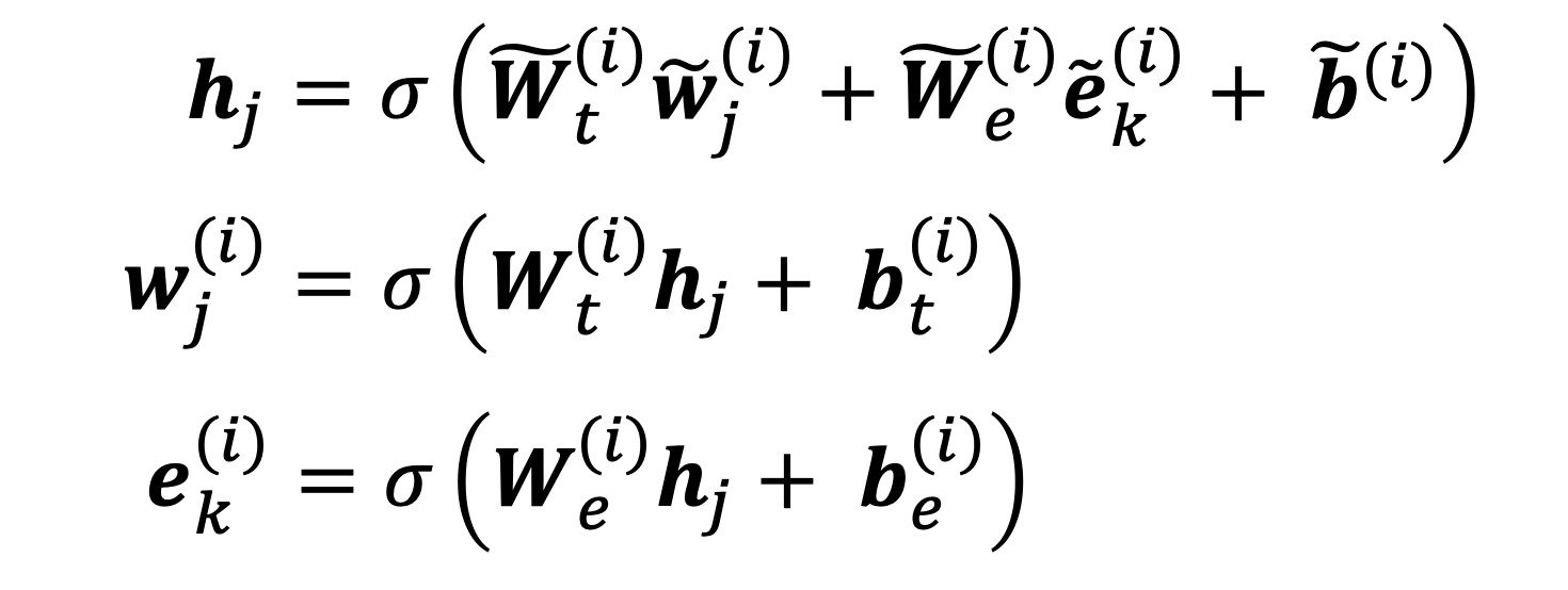
  $h_j=F(W_tw_j+W_Ee_k+b)$

ERNIE

architecture

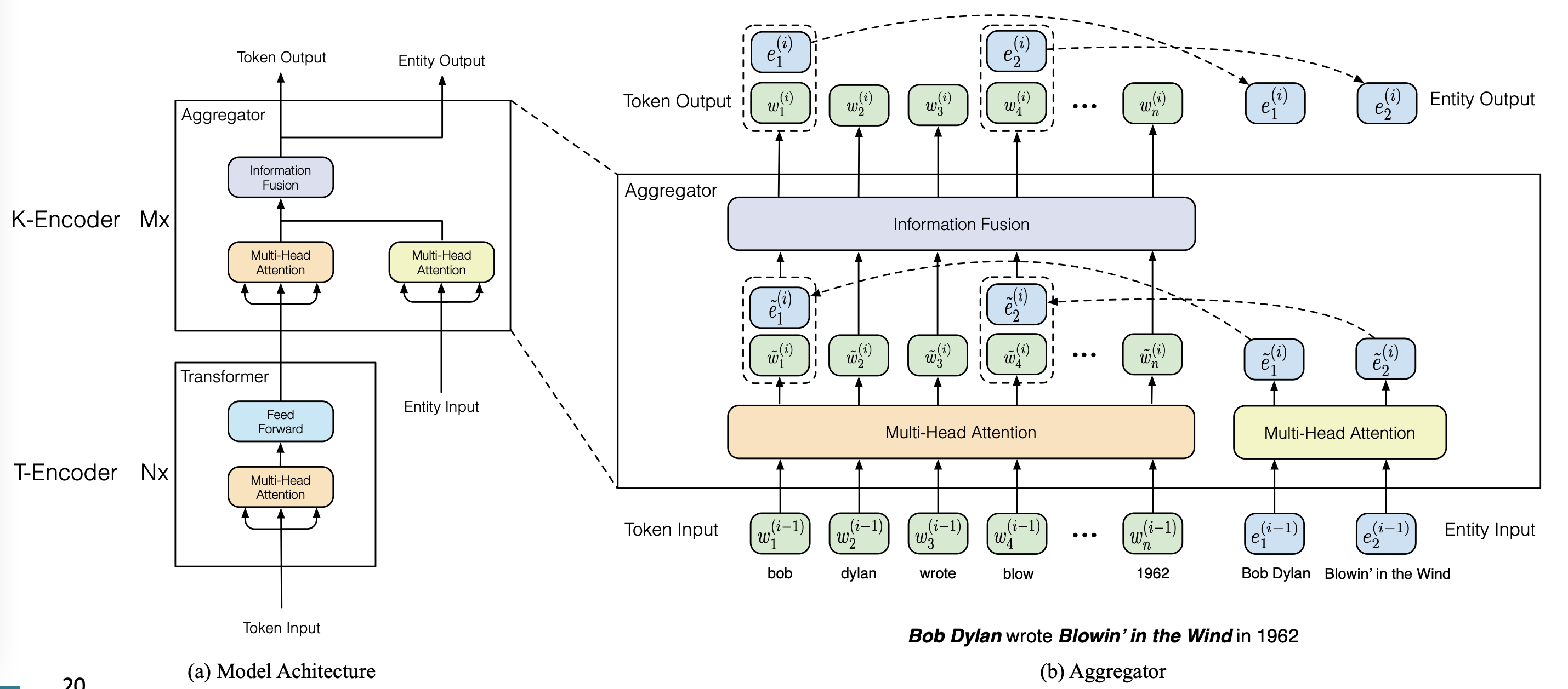
• text-encoder
  • multi-layer bidirectional Transformer
• knowledge encoder
  • 2 multi-head attention over entity embedding and token embedding
  • 1 fusion layer to combine
    

pretrain tasks

• BERT tasks
  • MLM
  • NSP
• knowledge pretraining task(dEA, denoising entity autoencoder)
  • 随机mask掉一个token-entity alignment，然后根据sequence中的实体预测出该token的相关entity
    $p(e_j|w_i)=\frac{exp(Ww_i\cdot e_j)}{\Sigma_{k=1}^{m}exp(Ww_i\cdot e_k)}$

$L_{ERNIE}=L_{MLM}+L_{NSP}+L_{dEA}$

strengths

• 通过fusion layer和dEA融合了entity和context

• 对知识驱动的下游任务提升很大

• remaining challenges

  • 需要带entity标注的数据作为输入，需要一个entity linker
  • 需要further pretrain

KnowBERT

• 核心思想：在BERT之外预训练一个entity linker
  $L_{KnowBERT}=L_{MLM}+L_{NSP}+L_{EL}$
• 在下游任务中，不需要额外的entity标注

KGLM

• 之前的方法依赖于预训练的entity embedding来从KB编码知识
• 需要更直接的方法来为LM提供额外知识

• solution：让模型可以直接访问三元组（key-value store）

• advantages

  • 可以更好地更新知识
  • 可解释性更强

• 核心思想：在KG上调整LM

• 利用entity的信息来预测下一word $P(x^{(t+1)},\epsilon^{(t+1)}|x^{(t)},\dots,x^{(1)},\epsilon^{(t)},\dots,\epsilon^{(1)})$
  $\epsilon^{(t)}$是t时刻提及的KG entities

architecture

• 在迭代时构建一个”local” KG
  • local KG——full KG的子集：只包含和sequence相关的entities
• next word有三类：
  • 已经在local KG中的related entity
    • 需要找到最高得分的head和relation
    • $P(e_h)=softmax(v_h\cdot h_t)$
    • 找到tail entity
    • 从entity扩展token
  • 不在local KG中的new entity
    • 在full KG中找到tail entity
  • 非entity
    • 退化
• 用LSTM的hidden state预测net word 的类型

KNN-LM

• 核心思想：学习句子间的similarity要比预测next word更容易，尤其对long-tail pattern更有效
  • 寻找k个相似句子
  • 从中检索相应的value（i.e. next word）
  • 将knn概率和LM概率结合

WKLM

• 之前的方法是从外部引入知识或使用额外的memory

• 将knowledge引入非结构文本

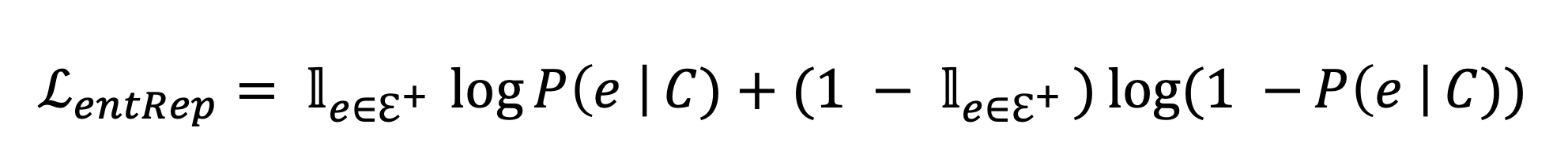
• 核心思想：训练模型去辨别知识的真伪

• 用同类型的其他entity替换，生成negative knowledge statement
• Loss：$L=L_{MLM}+L_{entRep}$，前者是token-level的，后者是entity-level的
  

Learn inductive biases through masking

ERNIE

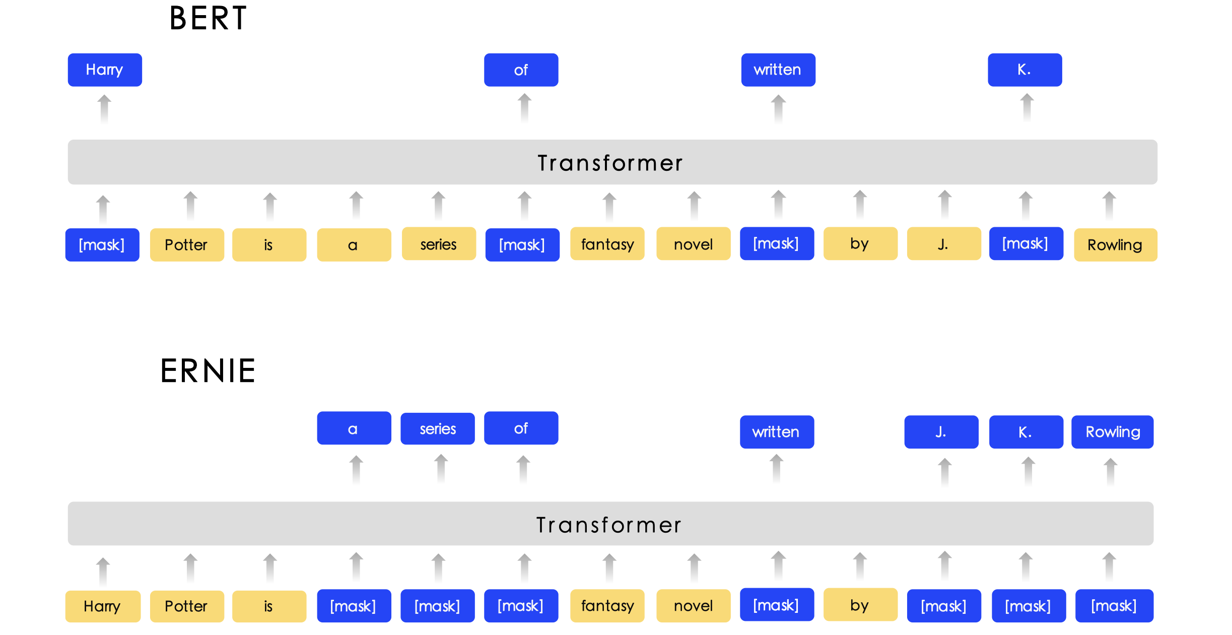
• 使用更有效的mask
  • phrase-level
  • entity-level

Salient span masking

• mask掉salient spans
  • named entities
  • dates